Practical on DAGs

# Install necessary packages if not already installed
required_pkgs <- c("dagitty", "ggplot2", "broom", "purrr", "dplyr", "data.table", "marginaleffects")
cran_repo <- "https://mirror.lyrahosting.com/CRAN/" # <- a CRAN mirror in the Netherlands, can select another one from here https://cran.r-project.org/mirrors.html

for (pkg in required_pkgs) {
  if (!requireNamespace(pkg, quietly = TRUE)) {
    install.packages(pkg, repos=cran_repo)
  }
}

suppressPackageStartupMessages({
  # Load packages
  library(purrr)
  library(broom)
  library(dagitty)
  library(ggplot2)
  library(dplyr)
  library(marginaleffects)
  library(data.table)
})

source(here::here("practicals", "21_dags", "_makedatas.R"))
datas <- make_datas()
birthw <- datas[['birthw']]

1 Exercise: making a DAG and specifying the correct adjustment set

In this example we’ll practice creating a DAG, and we’ll see how using the wrong DAG leads to the wrong analysis and wrong answers.

Our question is “what is the effect of maternal smoking during pregnancy on neonatal death within 3 months” (expressed as a difference in percentage risk for smoking / no smoking)

1.1 Birthweight data:

We’ll use the (simulated) dataset birthw with data on birthweight and survival of babies.

The birthw dataset contains the following variables:

• ageover35: Indicator mother’s age over 35 years (0 = age <= 35, 1 = age >35)
• smoking: Smoking status during pregnancy (0 = no, 1 = yes)
• lbwt: Low birth weight (0 = >=2500grams, 1 = < 2500grams)
• death: Neonatal death within 3 months (0 = no, 1 = yes)

The data can be downloaded here: birthw.csv

1.2 Create a DAG

1.2.1 Think of a DAG that may fit this data using the observed variables

Take a few minutes to create a DAG (collaboratively) (using e.g. dagitty.net)

1.2.2 Are there variables that may be missing in the data but are relevant?

If so, add them to the DAG, and indicate that they are unobserved

1.2.3 With your DAG, can the causal effect be estimated?

Use e.g. dagitty.net to create your DAG and see if there are ways to estimate the causal effect.

1.3 Analyse the data

Let’s try some analyses on the data. We’ll fit different logistic regression models with different covariates (independent variables). Specifically, fit a model with:

1. all observed covariates (fit_allobs)
2. only the smoking variable (fit_marginal)

These models give us estimates of (log) odds ratios for the independent variables. To translate a logistic regression model into differences in probabilities we use the avg_comparisons function from the marginaleffects package.

require(marginaleffects)

fit_allobs <- glm(death~., data=birthw, family="binomial")
fit_marginal <- glm(death~smoking, data=birthw, family="binomial")

avg_comparisons(fit_allobs, variables="smoking")

 Estimate Std. Error     z Pr(>|z|)    S  2.5 %  97.5 %
    -0.13     0.0179 -7.25   <0.001 41.1 -0.165 -0.0948

Term: smoking
Type: response
Comparison: 1 - 0

avg_comparisons(fit_marginal, variables="smoking")

 Estimate Std. Error    z Pr(>|z|)   S  2.5 % 97.5 %
   0.0808     0.0288 2.81  0.00502 7.6 0.0244  0.137

Term: smoking
Type: response
Comparison: 1 - 0

The effect estimates of fit_allobs and fit_marginal are quite different, they have different signs. How could this be explained? Which effect estimate do you think is more credible?

1.4 Assume a DAG

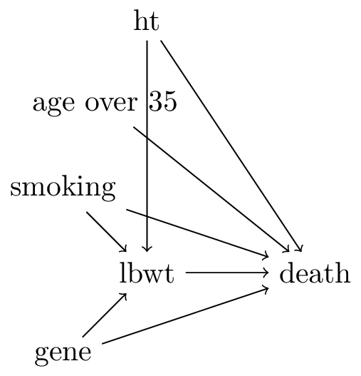
Assume the following DAG

Figure 1: DAG for smoking and death

In this DAG, there is another variable gene that influences both lbwt and death.

How does this DAG change the analysis? (tip: enter it in dagitty.net)

answer: the smoking-death relationship has no confounders, the marginal estimate is correct. Adjusting for lbwt ‘washes-out’ part of smoking’s effect because lbwt is a mediator. Also, lbwt is a collider between gene and smoking, and gene has a direct arrow into death. Conditioning on lbwt opens a bidirected path between smoking and gene, creating a new backdoor path. So there are two reasons not to condition on lbwt: it is a mediator and a collider with an unmeasured variable

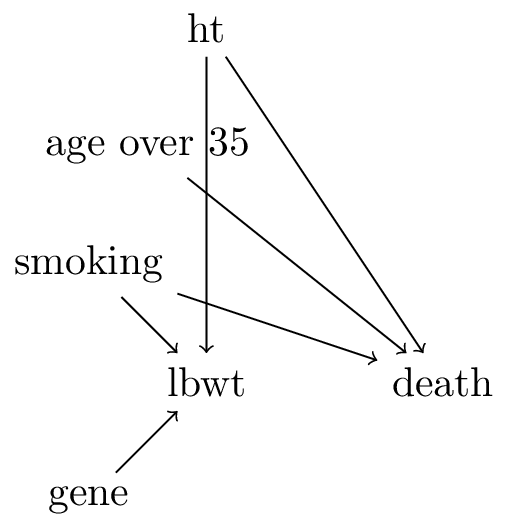
See this other DAG on the smoking question

Figure 2: birthweight DAG 2

Given the DAG in Figure 2, see the following regression model

fit2 <- glm(death~smoking+ht+ageover35, data=birthw, family=binomial)

Assuming no parametric form bias, will this lead to an unbiased causal effect estimate?

answer: yes this is a correct analysis. lbwt is still a collider, but it does not open any new back-door paths because gene no longer has a direct effect on death and all variables other than smoking that do have such an arrow are in the conditioning set (ageover35,ht) so these paths are blocked

2 DAG assumptions: conditional independencies and strength of assumptions

DAGs imply (conditional) indepencies. These can be checked with data.

See the DAGs in Figure 3.

(a) collider

(b) chain

(c) confounded

Figure 3

What independencies are implied by the DAGs?

answer:

• Figure 3 (a): \(X \perp Y\)
• Figure 3 (b): \(X \perp Y | M\)
• Figure 3 (c): none

We generated datasets according to each DAG named df1, df2 and df3, but forgot what dataset corresponded to what DAG.

Assume linear models with Gaussian error terms for all variables, how would you test the conditional independencies to figure out what DAG corresponds to what dataset?

summary(lm(y~x, data=df1))
summary(lm(y~x+z, data=df1))

summary(lm(y~x, data=df2))
summary(lm(y~x+z, data=df2))

summary(lm(y~x, data=df3))
summary(lm(y~x+z, data=df3))

The datasets are downloadable here:

data	link
df1	data1.csv
df2	data2.csv
df3	data3.csv

See the results of the analyses summarized below in Table 1

dfnames <- c("df1", "df2", "df3")
fits_marginal    <- map(dfnames, function(dfname) lm(y~x, data=datas[[dfname]]))
fits_conditional <- map(dfnames, function(dfname) lm(y~x+z, data=datas[[dfname]]))
names(fits_marginal) <- dfnames
names(fits_conditional) <- dfnames

results_marginal <- map(fits_marginal, broom::tidy) |> rbindlist(idcol="dataset")
results_conditional <- map(fits_conditional, broom::tidy) |> rbindlist(idcol="dataset")
results_df <- rbindlist(list(
  marginal = results_marginal,
  conditional = results_conditional
), idcol="analysis")
results_df[, rformula:=ifelse(analysis=="marginal", "lm(y~x)", "lm(y~x+z)")]

dcast(results_df[term%in%c("x")], dataset ~ rformula, value.var="p.value")

Table 1: P-values for coefficient of variable x in linear regression model

What is the conclusion regarding what dataset corresponds to what DAG?

answer:

• df1: Figure 3 (b)
• df2: Figure 3 (c)
• df3: Figure 3 (a)

2.1 Non-coding questions

2.1.1 Strength of Assumptions

(a) DAG

(b) DAG

(c) DAG

Figure 4

What is the correct ordering of the strength of assumptions in the above DAGs, starting with the strongest assumption

answer: Figure 4 (b) > Figure 4 (c) > Figure 4 (a)

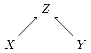
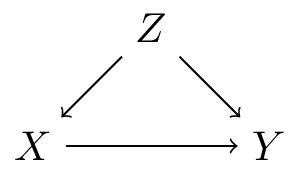
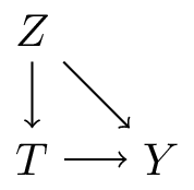
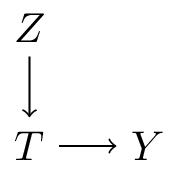
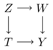
Figure 4 (b) is stronger than Figure 4 (c) as in the latter, it could be that the effects through \(W\) are all absent (remember that the presence of an arrow from A to B implies a possible effect of A on B)

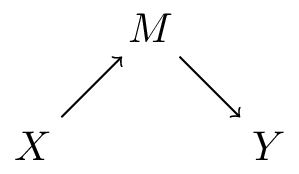
Figure 4 (c) is stronger than Figure 4 (a) as in the first, Z can only affect Y through T and W, whereas in Figure 4 (a) Z can effect Y through T and can effect Y through other paths (e.g. W)

see also the lecture on DAGs

2.1.2 RCTs

According to the DAG framework, why are RCTs especially fit for causal questions?

1. they are often infeasible and unethical
2. they sample data from the target distribution
3. they have better external validity than observational studies
4. randomization balances confounders

Which answers are true?

answer: 2.

See also the DAG lecture

Context:

1. This is often said of RCTs but has no direct bearing on why they are special for causal inference
2. Remember that the target distribution has no arrows going in to the treatment variable, this is what we get in a RCT
3. RCTs are often critiqued as having poor external validity, because they may recruit non-random subpopulations from the target population
4. This is a subtle point, but RCTs have no confounders as there are no common causes of the treatment and the outcome. Variables that are confounders in observational studies are prognostic factors in RCTs, as they (by definition of being a confounder in an observational study) influence the outcome, but not the treatment in the RCT. Randomization balances the distribution of prognostic factors between treatment arms in expectation. In a particular RCT, observed (and unobserved) prognostic factors will always have some random variation between treatment arms. This does not reduce the validity of the RCT in terms of bias. This variation is reflected in the standard error of the estimate. In some cases, adjusting for known prognostic factors in RCTs may reduce the variance of the treatment estimate (i.e. narrowing the confidence interval), but this is an entire discussion on its own.

3 Confounder adjustment with Daggity

In this exercise we will use the dagitty package for creating and manipulating DAGs.

3.1 Creating and Visualizing a DAG

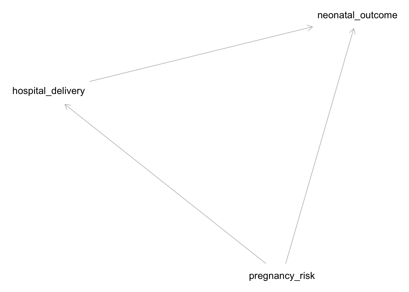
Let’s create a DAG for the pregnancy example:

# Define the DAG
dag <- dagitty("dag {
  pregnancy_risk -> hospital_delivery
  pregnancy_risk -> neonatal_outcome
  hospital_delivery -> neonatal_outcome
}")

# Plot the DAG
plot(dag)

Plot coordinates for graph not supplied! Generating coordinates, see ?coordinates for how to set your own.

This DAG assumes that pregnancy risk influences both the likelihood of hospital delivery and neonatal outcomes, and that hospital delivery affects neonatal outcomes.

3.1.1 Simulating Data

We will simulate data based on the DAG structure:

set.seed(123)

n <- 10000

# Simulate variables
pregnancy_risk <- rbinom(n, 1, 0.3)  # 30% high risk
hospital_delivery <- rbinom(n, 1, 0.5 + 0.3 * pregnancy_risk)  # 50% baseline + 30% if high risk
neonatal_outcome <- rbinom(n, 1, 0.8 - 0.3 * pregnancy_risk + 0.15 * hospital_delivery)  # outcome affected by both

# Create a data frame
df <- data.table(pregnancy_risk, hospital_delivery, neonatal_outcome)

3.1.2 Analyzing the Data

Check the relationships in the data:

# Summary statistics
summary(df)

 pregnancy_risk   hospital_delivery neonatal_outcome
 Min.   :0.0000   Min.   :0.0000    Min.   :0.0000  
 1st Qu.:0.0000   1st Qu.:0.0000    1st Qu.:1.0000  
 Median :0.0000   Median :1.0000    Median :1.0000  
 Mean   :0.2952   Mean   :0.5859    Mean   :0.7982  
 3rd Qu.:1.0000   3rd Qu.:1.0000    3rd Qu.:1.0000  
 Max.   :1.0000   Max.   :1.0000    Max.   :1.0000  

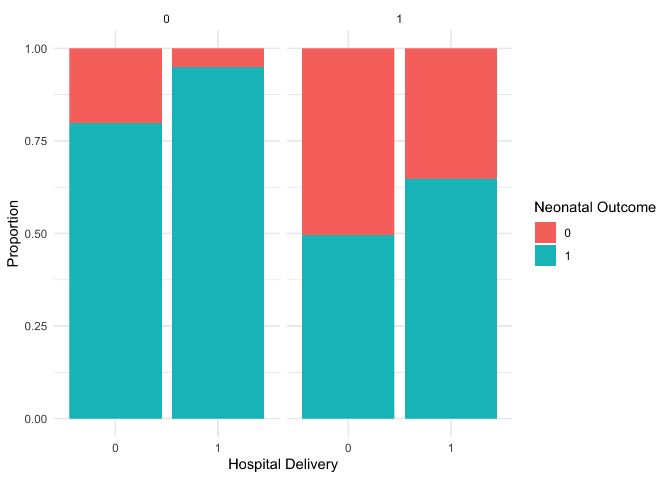
# Plot the data
ggplot(df, aes(x = factor(hospital_delivery), fill = factor(neonatal_outcome))) +
  geom_bar(position = "fill") +
  facet_grid(~ pregnancy_risk) +
  labs(x = "Hospital Delivery", y = "Proportion", fill = "Neonatal Outcome") +
  theme_minimal()

3.1.3 Causal Inference Using DAGs

Let’s use the DAG to determine what to condition on to estimate the causal effect of hospital delivery on neonatal outcomes:

# Identify adjustment set using DAGitty
adjustmentSets(dag, exposure = "hospital_delivery", outcome = "neonatal_outcome")

{ pregnancy_risk }

The output will suggest which variables to condition on to estimate the causal effect correctly. In this case, we need to condition on pregnancy_risk.

3.1.4 Estimating the Causal Effect

Estimate the causal effect using a regression model:

# Fit a regression model
model <- glm(neonatal_outcome ~ hospital_delivery + pregnancy_risk, family = binomial, data = df)

# Summarize the model
summary(model)

Call:
glm(formula = neonatal_outcome ~ hospital_delivery + pregnancy_risk, 
    family = binomial, data = df)

Coefficients:
                  Estimate Std. Error z value Pr(>|z|)    
(Intercept)        1.48278    0.04048   36.63   <2e-16 ***
hospital_delivery  1.15677    0.06169   18.75   <2e-16 ***
pregnancy_risk    -1.91810    0.06177  -31.05   <2e-16 ***
---
Signif. codes:  0 '***' 0.001 '**' 0.01 '*' 0.05 '.' 0.1 ' ' 1

(Dispersion parameter for binomial family taken to be 1)

    Null deviance: 10057.8  on 9999  degrees of freedom
Residual deviance:  8896.9  on 9997  degrees of freedom
AIC: 8902.9

Number of Fisher Scoring iterations: 5

3.1.5 Drawing Conclusions

Interpret the model’s output to understand the effect of hospital delivery on neonatal outcomes, controlling for pregnancy risk.

avg_comparisons(model, variables="hospital_delivery")

 Estimate Std. Error    z Pr(>|z|)     S 2.5 % 97.5 %
    0.166     0.0084 19.8   <0.001 286.7  0.15  0.183

Term: hospital_delivery
Type: response
Comparison: 1 - 0

Is this odds ratio a correct estimate of the causal effect?

answer: no

hint: compare the structural equation used in generating the data with the statistical analysis

This linear probability structural equation is not well-approximated by a linear logistic model (i.e. without interaction terms). We can model the outcome without making parametric assumptions by including an interaction term, and then extract the risk difference using avg_comparisons from package marginaleffects.

The correct estimate is given by:

full_model <- glm(neonatal_outcome~hospital_delivery*pregnancy_risk, family=binomial, data=df)
avg_comparisons(full_model, variables="hospital_delivery")

 Estimate Std. Error    z Pr(>|z|)     S 2.5 % 97.5 %
    0.152    0.00869 17.5   <0.001 225.2 0.135  0.169

Term: hospital_delivery
Type: response
Comparison: 1 - 0