Causal Directed Acylic Graphs
introduction
2024-08-06
Example task: are hospital deliveries good for babies?


New question: hernia
- for a patient with a hernia, will they be able to walk sooner when recovering at home or when recovering in a hospital?
- observed data: location, recovery, bed-rest


Causal Directed Acyclic Graphs
diagram that represents our assumptions on causal relations
- nodes are variables
- arrows (directed edges) point from cause to effect

- when used to convey causal assumptions, DAGs are ‘causal’ DAGs1
Making DAGs for our examples:
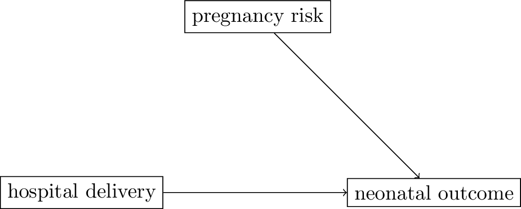
The pregnancy DAG
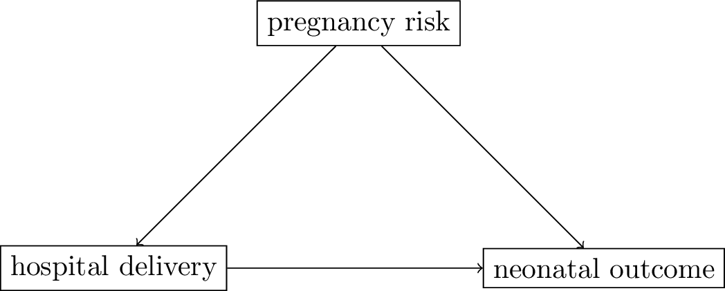
- assumptions:
- women with high risk of bad neonatal outcomes (
pregnancy risk) are referred to the hospital for delivery - hospital deliveries lead to better outcomes for babies as more emergency treatments possible
- both
pregnancy riskandhospital deliverycauseneonatal outcome
- women with high risk of bad neonatal outcomes (
- the other variable
pregnancy riskis a common cause of the treatment (hospital delivery) and the outcome (this is called a confounder)
Making DAGs for our examples:
The hernia DAG
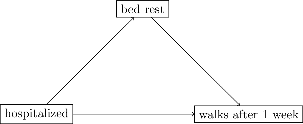
- assumptions:
- patients admitted to the hospital keep more
bed restthan those who remain at home bed restleads to lower recovery times thus less walking patients after 1 week
- patients admitted to the hospital keep more
- the other variable
bed restis a mediator between the treatment (hospitalized) and the outcome
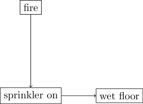
DAGs convey two types of assumptions:
causal direction and conditional independence
- causal direction: what causes what?
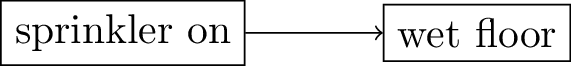
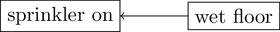
- read Figure 4 as
sprinkler onmay (or may not) causewet floorwet floorcannot causesprinkler on
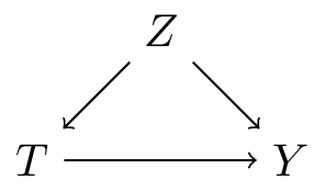
Basic DAG patterns: fork
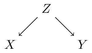
- \(Z\) causes both \(X\) and \(Y\) (common cause / confounder)
- \(Z\) = sun rises, \(X\) = rooster crows, \(Y\) = temperature rises
- \(X \mathrel{\not\!\perp} Y\) (i.e. \(X\) and \(Y\) are dependent)
- \(X \perp Y | Z\) (conditioning on the sun rising, the rooster crowing has no information on the temperature)
- \(Z \to X\) is a back-door: a path between \(X\) and \(Y\) that starts with an arrow into \(X\)
- typically want to adjust for \(Z\) (see later 6.4)
Basic DAG patterns: chain
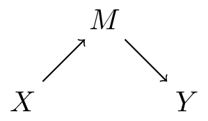
- \(M\) mediates effect of \(X\) on \(Y\)
- \(X\): student signs up for causal inference course, \(M\): student studies causal inference, \(Y\): student understands causal inference
- \(X \mathrel{\not\!\perp} Y\) (i.e. \(X\) and \(Y\) are dependent)
- \(X \perp Y | M\)
- typically do not want to adjust for \(M\) when estimating total effect of \(X\) on \(Y\)
Basic DAG patterns: collider
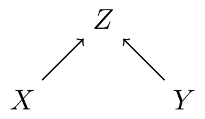
- \(X\) and \(Y\) both cause \(Z\)
- \(X \perp Y\) (but NOT when conditioning on \(Z\))
- often do not want to condition on \(Z\) as this induces a correlation between \(X\) and \(Y\)
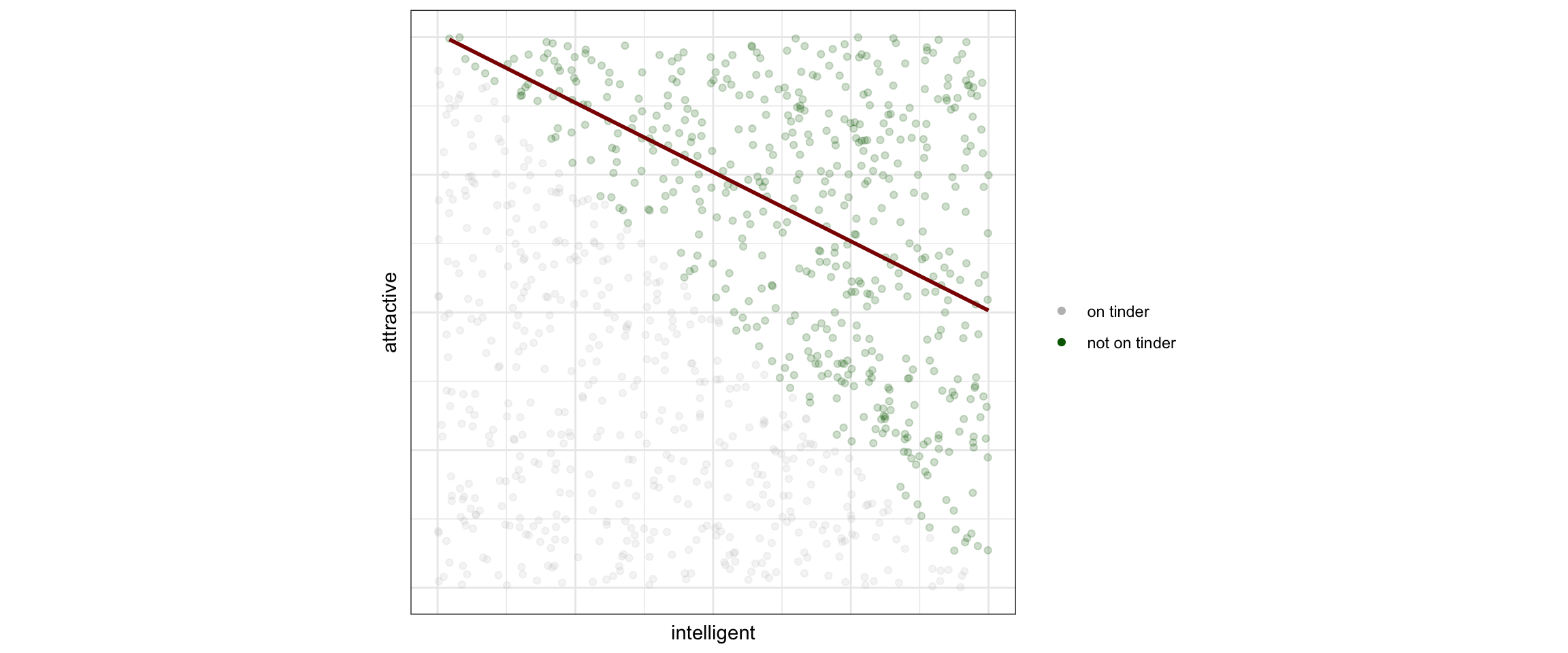
Collider bias - Tinder
DAGs convey two types of assumptions:
causal direction and conditional independence
- conditional indepence (e.g. exclusion of influence / information)
DAGs are ‘non-parametric’
They relay what variable ‘listens’ to what, but not in what way
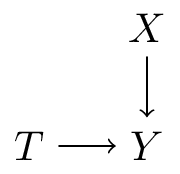
- this DAG says \(Y\) is a function of \(X,T\) and external noise \(U_Y\), or:
- \(Y = f_Y(X,T,U_Y)\)
- in the next lecture we’ll talk more about these ‘structural equations’
DAGs are ‘non-parametric’
They relay what variable ‘listens’ to what, but not in what way
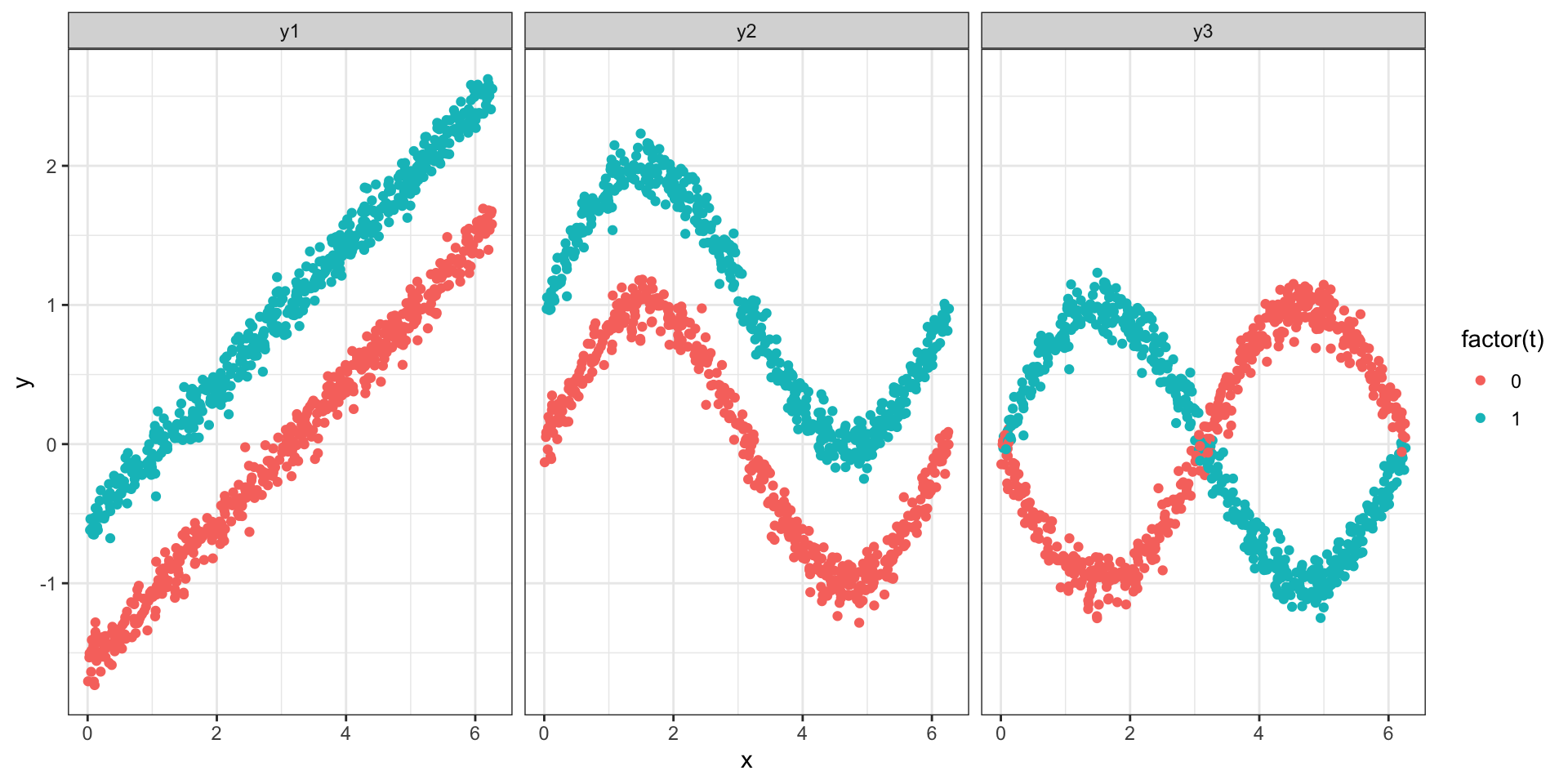
- \(Y = T + 0.5 (X - \pi) + \epsilon\) (linear)
- \(Y = T + \sin(X) + \epsilon\) (non-linear additive)
- \(Y = T * \sin(X) - (1-T) \sin(x) + \epsilon\) (non-linear + interaction)
Mini Quiz
Google Form https://bit.ly/dagquiz

The DAG definition of an intervention
assume this is our DAG for a situation and we want to learn the effect \(T\) has on \(Y\)
- in the graph, intervening on variable \(T\) means removing all incoming arrows
- this assumes such a modular intervention is possible: i.e. leave everything else unaltered
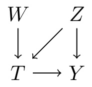
- which means \(T\) does not listen to other variables anymore, but is set at a particular value, like in an experiment
- imagining this scenario requires a well-defined treatment variable (akin to consistency)
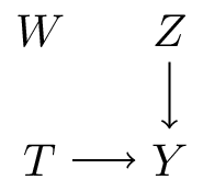
Intervention example: hospital deliveries
- this is called graph surgery because we cut all the arrows going to the treatment (hospital delivery)
DAGs imply a causal factorization of the joint distribution
\[\begin{align} P(Y,T,Z) &= P(Y|T,Z)P(T,Z) \\ &= P(Y|T,Z)P(T|Z)P(Z) \end{align}\]
- 2 times the product rule
- If this looks complicated: just follow the arrows, starting with variables with no incoming arrows
Intervention as graph surgery
Why is the causal factorization special?

\[\begin{align} P_{\text{obs}}(Y,T,Z) &= P(Y|T,Z)\color{red}{P(T|Z)}P(Z) \end{align}\]
\[\begin{align} P_{\text{int}}(Y,T,Z) &= P(Y|T,Z)\color{green}{P(T)}P(Z) \end{align}\]
- in the causal factorization, intervening on \(T\) means changing only one of the conditionals in the factorization, the others remain the same
- this is what is meant with a modular intervention
Intervention as graph surgery
Changed distribution
\[\begin{align} P_{\text{obs}}(Y,T,Z) &= P(Y|T,Z)\color{red}{P(T|Z)}P(Z) \\ P_{\text{obs}}(Y|T) &= \sum_{z} P(Y|T,Z=z)P(Z=z|T) \end{align}\]
\[\begin{align} P_{\text{int}}(Y,T,Z) &= P(Y|T,Z)\color{green}{P(T)}P(Z) \\ P_{\text{int}}(Y|T) &= \sum_{z} P(Y|T,Z=z)P(Z=z|T) \\ &\class{fragment}{= \sum_{z} P(Y|T,Z=z)\color{green}{P(Z)}} \\ &\class{fragment}{= P(Y|\text{do}(T))} \end{align}\]
Intervention as graph surgery - changed distribution
\[P_{\text{obs}}(Y|T) = \sum_{z} P(Y|T,Z=z)\color{red}{P(Z=z|T)}\]
\[P_{\text{int}}(Y|T) = \sum_{z} P(Y|T,Z=z)\color{green}{P(Z=z)} \qquad(1)\]
- in \(P_{\text{obs}}\), \(P(Z|T) \color{red}{\neq} P(Z)\)
- in \(P_{\text{int}}\), \(P(Z|T) \color{green}{=} P(Z)\)
- thereby \(P_{\text{obs}}(Y|T) \neq P_{\text{int}}(P(Y|T)) = P(Y|\text{do}(T))\)
- seeing is not doing
- looking at Equation 1, we can compute these from \(P_{\text{obs}}\)! (this is what is called an estimand)
Back to example 1
Seeing
| location | |||
|---|---|---|---|
| home | hospital | ||
| risk | low | 648 / 720 = 90% | 19 / 20 = 95% |
| high | 40 / 80 = 50% | 144 / 180 = 80% | |
| marginal | 688 / 800 = 86% | 163 / 200 = 81.5% |
- seeing: \(P(\text{outcome}|\text{location}) = \sum_{\text{risk}} P(\text{outcome}|\text{location},\text{risk})P(\text{risk}|\text{location})\)
- \(P(\text{risk}=\text{low} | \text{location} = \text{hospital})=10\%\)
- \(P(\text{risk}=\text{low} | \text{location} = \text{home})=90\%\)
\[\begin{align} P(\text{outcome}|\text{location} = \text{hospital}) &= 95 * 0.1 + 80 * 0.9 = 81.5\% \\ P(\text{outcome}|\text{location} = \text{home}) &= 90 * 0.9 + 50 * 0.1 = 86\% \end{align}\]
- conclusion: deliveries in the hospital had worse neonatal outcomes
Back to example 1
| location | |||
|---|---|---|---|
| home | hospital | ||
| risk | low | 648 / 720 = 90% | 19 / 20 = 95% |
| high | 40 / 80 = 50% | 144 / 180 = 80% | |
| marginal | 688 / 800 = 86% | 163 / 200 = 81.5% |
- estimand: \(P(\text{outcome}|\text{do}(\text{location})) = \sum_{\text{risk}} P(\text{outcome}|\text{location},\text{risk})P(\text{risk})\)
- \(P(\text{risk}=\text{low})=74\%\)
\[\begin{align} P(\text{outcome}|\text{do}(\text{hospital})) &= 95 * 0.74 + 80 * 0.26 = 91.1\% \\ P(\text{outcome}|\text{do}(\text{home})) &= 90 * 0.74 + 50 * 0.26 = 79.6\% \end{align}\]
- conclusion: sending all deliveries to the hospital leads to better neonatal outcomes
Back to example 2
- removing all arrows going in to \(T\) results in the same DAG
- so \(P(Y|T) = P(Y|\text{do}(T))\)
- i.e. use the marginals
The gist of observational causal inference
is to take data we have to make inferences about data from a different distribution (i.e. the intervened-on distribution)
- causal inference frameworks provide a language to express assumptions
- based on these assumptions, the framework tells us whether such an inference is possible
- this is often referred to as is the effect identified
- and provide formula(s) for how to do so based on the observed data distribution (estimand(s))
- (one could say this is essentially assumption-based extrapolation, some researchers think this entire enterprise is anti-scientific)
- not yet said: how to do statistical inference to estimate the estimand (much can still go wrong here)
- can also be part of identification, see the following lecture on SCMs
When life gets complicated / real
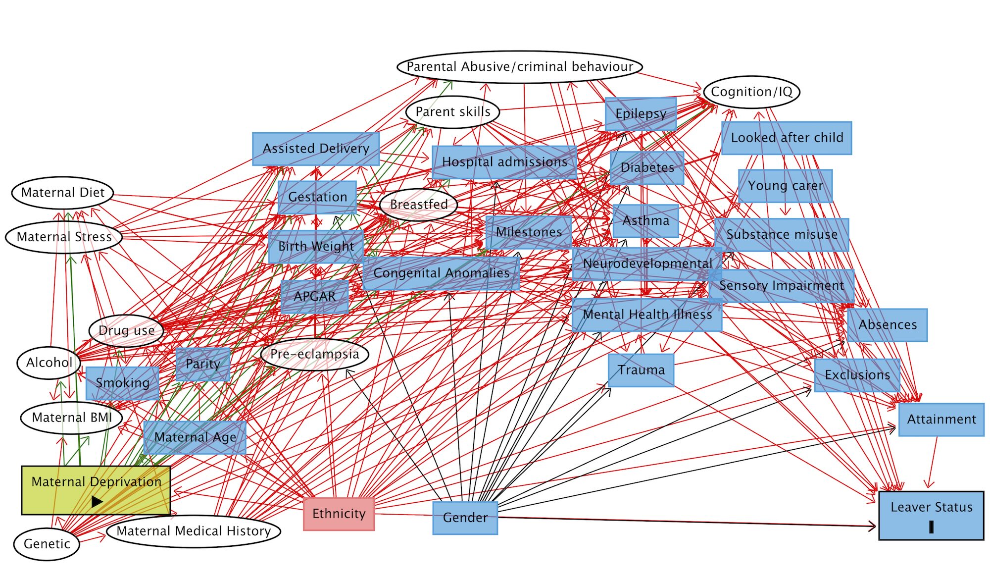
Bogie, James; Fleming, Michael; Cullen, Breda; Mackay, Daniel; Pell, Jill P. (2021). Full directed acyclic graph.. PLOS ONE. Figure. https://doi.org/10.1371/journal.pone.0249258.s003
d-separation (directional-separation)
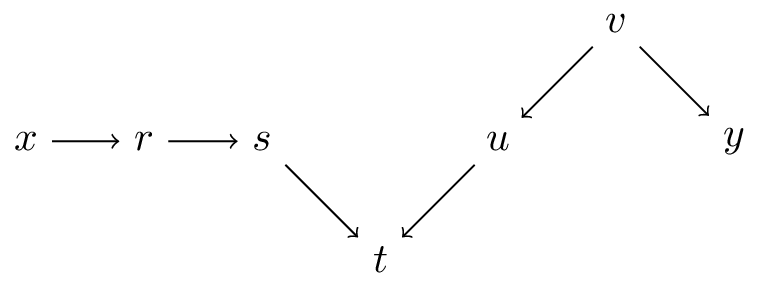
paths
- a path is a set of nodes connected by edges (\(x \ldots y\))
- a directed-path is a path with a constant direction (\(x \dots t\))
- an unblocked-path is a path without a collider (\(t \ldots y\))
- a blocked-path is a path with a collider (\(s,t, u\))
- d(irectional)-separation of \(x,y\) means there is no unblocked path between them
d-separation when conditioning
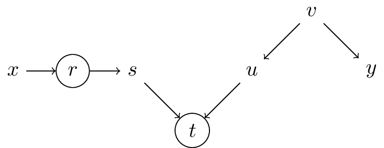
paths with conditioning variables \(r\), \(t\)
- conditioning on variable:
- when variable is a collider: opens a path (\(t\) opens \(s,t,u\) etc.)
- otherwise: blocks a path (e.g. \(r\) blocks \(x,r,s\))
- conditioning set \(Z=\{r,t\}\): set of conditioning variables