f_surgery <- function(u_surgery) { # pa_surgery = {}
  u_surgery
}
f_los <- function(surgery, u_los) { # pa_los = {surgery}
  surgery + u_los
}
f_survival <- function(surgery, los, u_survival) { # pa_survival = {sugery, los}
  survival = los - 2 * surgery + u_survival
}

scm1 <- function(u_surgery, u_los, u_survival) {
  surgery  = f_surgery(u_surgery)
  los      = f_los(surgery, u_los)
  survival = f_survival(surgery, los, u_survival)
  c(surgery=surgery, los=los, survival=survival)
}
scm1(2, 1, 5)Structural Causal Models
introduction
2024-08-06
In this lecture: structural causal models (SCMs)
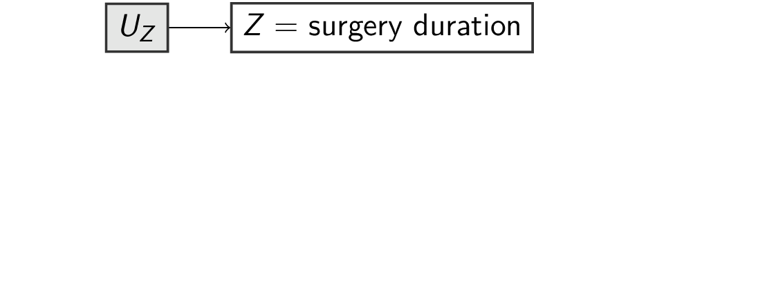
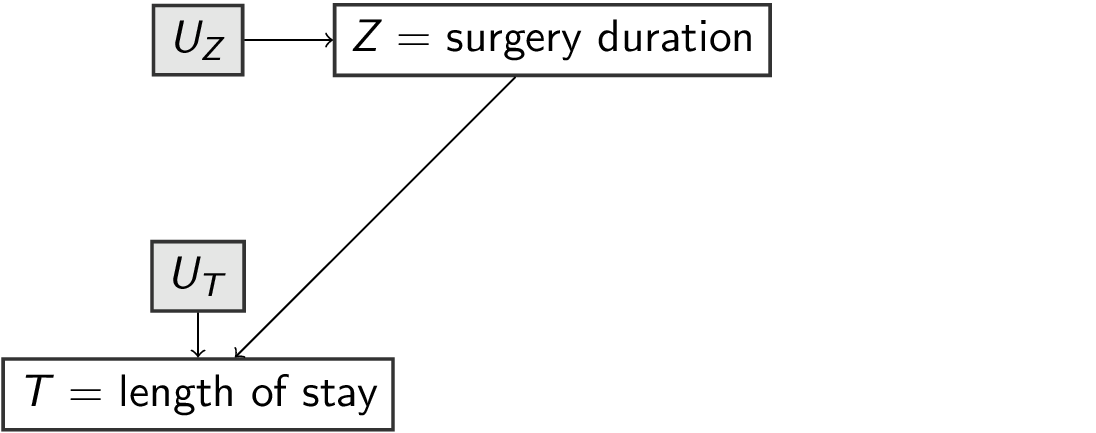
\[\begin{align} U_Z, U_T, U_Y &\sim p(U) \\ Z &= f_Z(U_Z) \\ T &= f_T(Z,U_T) \\ Y &= f_Y(T,Z,U_Y) \end{align}\]


Recursive Structural Causal Models imply a Directed Acyclic Graph
An SCM is recursive, i.e. acyclic when following the chain of parents, you never end up at the same variable twice
Recursive Structural Causal Models imply a Directed Acyclic Graph
An SCM is recursive, i.e. acyclic when following the chain of parents, you never end up at the same variable twice
Recursive Structural Causal Models imply a Directed Acyclic Graph
An SCM is recursive, i.e. acyclic when following the chain of parents, you never end up at the same variable twice
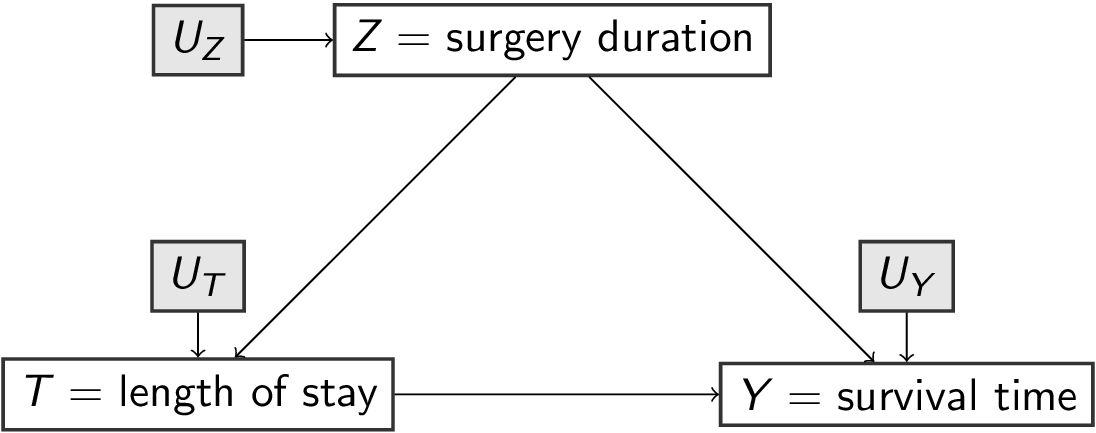
scm1 (without specifying the f_s) and the DAG are equivalent (they describe the same knowledge of the world)
for the remainder, we assume recursiveness
Submodel and Effect of Action as a mutilated DAG
In scm1 replace f_los with a specific value, e.g. 7 days (notation: \(M_x\))
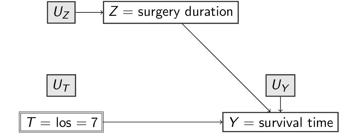
The DAG describes a submodel where \(T\) no longer ‘listens’ to any variables but is controlled to be equal to a specific value (e.g. 7)
The Effect of Action \(do(X=x)\) is defined as the submodel \(M_x\).
Specifying a distribution for exogenous variables U
- Exogenous variables
Urepresent random variation in the world. - We can specify a distribution for them (e.g. Gaussian, Uniform)
 u_surgery      u_los u_survival
5.299693 4.308564 12.199266 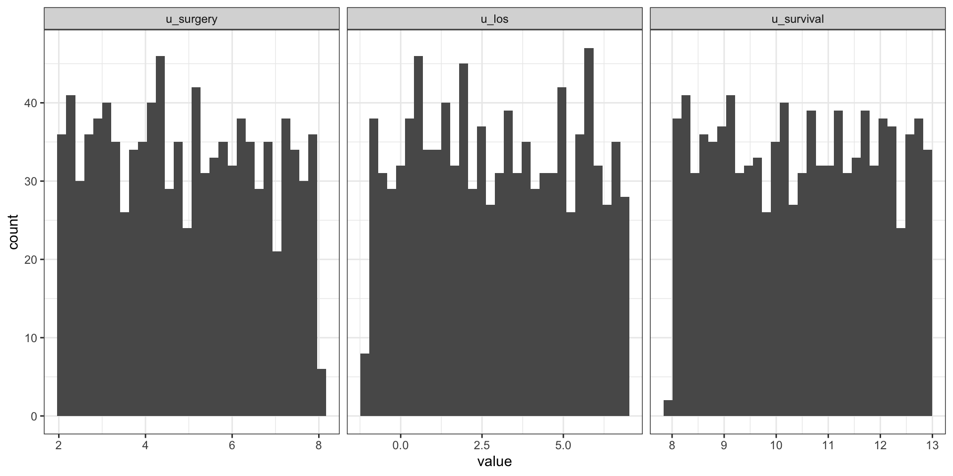
A Probabilistic Causal Model is a SCM with a distribution over U
 u_surgery      u_los u_survival    surgery        los   survival
3.019182 1.401587 10.914728 3.019182 4.420770 9.297133 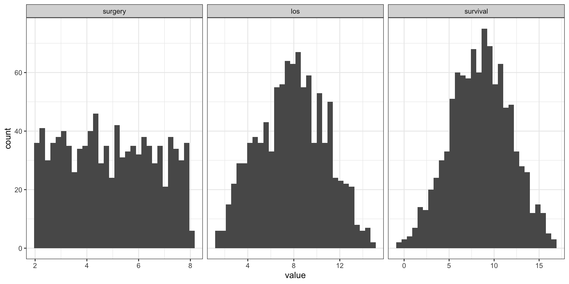
Idenfitication in pictures
Someone killed the priest (†), we want to know who-dunnit (\(=Q\))
Based on prior knowledge we have 5 suspects (all the SCMs compatible with our DAG)
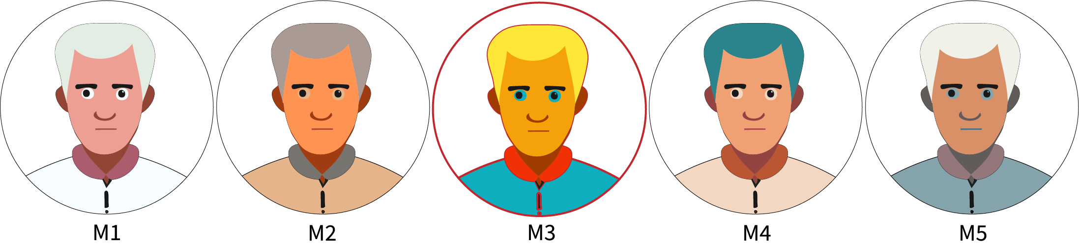
If we had full data, we would know it was \(M_3\)
Idenfitication in pictures
Someone killed the priest (†) , we want to know who-dunnit (\(=Q\))
Based on prior knowledge on 5 suspects (all the SCMs compatible with our DAG)

If we had full data, we would have know it was \(M_3\)
Unfortunately, it was dark an we only got a gray-scale image of the perpetrator
All our suspects (models) lead to the same partial observations
Based on observed data and assumptions we cannot identify the answer to our question \(Q\),
i.e. multiple models with different answers for \(Q\) fit the observed data equally well
Not identified vs estimand
The backdoor adjustment in this DAG means the correct estimand is:
\[\begin{align} P(Y|\text{do}(T)) &= \sum_{z} P(Y|T,z)P(Z=z) \end{align}\]
- If we did not observe \(Z\), we could still come up with a latent-variable model for \(Z\) and a model for \(Y|T,Z\) and get a value.
- However, we can formulate multiple distinct latent variable models that each yield a different treatment effect (i.e. the output of the estimand)
- But these latent variable models all fit the observed data equally well
- So we cannot identify the treatment effect
Seeing is not doing
\[\begin{align} P(Y|T) &= \sum_{z} P(Y|T,z)P(Z=z|T) \\ &=^2 \sum_{z} P(Y|T,z)P(Z=z) \end{align}\]
- \(P(Y|\text{do}(T)) \neq P(Y|T)\) is Pearl’s definition of confounding (def 6.2.1)
- this shows why RCTs are special (i.e. no backdoor paths into \(T\))
Adam versus Zoe
- Average causal effects in subgroup with
surgery=4:- 3-days LOS: 5.5
- 7-days LOS: 9.5

- what do we expect for Adam and Zoe if they would have been kept in the hospital for 7 days?