Marginally Constrained Models and Treatment Offset Models
CATE estimation from observational data plus randomized evidence
Department of Data Science Methods, Julius Center, University Medical Center Utrecht
2026-06-23
Treatment decisions need individualized effects
Treatment decisions compare two potential outcomes: \[Y_1 \quad \text{versus} \quad Y_0\]
The clinically useful quantity is often the conditional average treatment effect: \[\tau(x) = E(Y_1 - Y_0 \mid X=x)\]
Patients and care-givers prefer this to be on an absolute (probability) scale (Murray et al. 2018)
Example: cardiovascular risk with or without cholesterol-lowering medication, given a patient’s history.
Why CATE estimation is hard
- Randomized controlled trials estimate average treatment effects.
\[\text{ATE} = E[\tau(x)]\]
- Estimating highly conditional effects in trials is expensive and often underpowered.
- Observational data are large and rich, but treatment assignment is confounded.
So the question is:
Can we combine observational outcome models with treatment effects known from randomized trials?
Effect measures matter
For binary outcomes, trials may report several valid causal summaries:
\[ \begin{aligned} \text{risk difference} &= P(Y_1=1)-P(Y_0=1),\\ \text{risk ratio} &= \frac{P(Y_1=1)}{P(Y_0=1)},\\ \text{odds ratio} &= \frac{\text{odds}(Y_1=1)} {\text{odds}(Y_0=1)}. \end{aligned} \]
(and their conditional variants)
Relative treatment effects tend to be more stable
- Empirical observation: meta-analyses group together different trials with often (slightly) different underlying populations, from different centers etcetera
- Meta-analyses report a weighted average aggregated treatment effect, alongside an estimate of residual heterogeneity of treatment effects across studies (in random effects meta-analysis)
- When averaging effects, (odds and risk)-ratios tend to show lower heterogeneity \(\rightarrow\) more stability across settings, are better transportable (Engels et al. 2000)
Combining RCT data with observational data requires an assumption of transportability, we study transportability of the odds-ratio, assuming we know it from an external RCT
Constant relative effects still variable absolute effects
- If we assume a constant odds ratio for treatment
- If \(\mathrm{OR}_T\) is constant, the absolute risk reduction (\(\tau\)) depends on baseline (untreated) risk.
\[ E(Y_0\mid X=x) \quad \Longrightarrow \quad \tau(x) = \text{odds}^{-1}(\text{OR}_T \text{odds}(Y_0 | X)) - E(Y_0\mid X=x) \]
- If we can estimate the untreated baseline risk conditional on \(X\) from observational data, then we can derive the treated risk and the CATE.
- Unfortunately, estimating \(E[Y_0|X]\) in general requires causal assumptions (unconfoundedness, positivity, consistency)
Offset models
An offset model fixes the treatment coefficient to the value known from randomized evidence and estimates the remaining parameters from observational data.
For a logistic outcome model:
\[ \mathrm{logit}\{P(Y=1\mid X=x,T=t)\} = \beta_0 + \beta_x^\top x + \beta_t t. \]
The usual offset approach plugs in \(\beta_t=\log(\mathrm{OR}_T^{RCT})\).
What the offset promises
- Use the rich covariates and large sample size of observational data.
- Avoid estimating the treatment effect from confounded treatment assignment.
- Produce baseline risk and treated risk from a single fitted model.
- Then derive CATEs under a constant relative treatment effect assumption.
This is already close to what some clinical prediction tools do in practice Alaa et al. (2021), some of which are recommended for use by clinical guidelines (Cardoso et al. 2019)
Unanswered question
assume a model exists, such that \[ \mathrm{logit}\{P(Y=1\mid X=x,T=t)\} = \beta_0 + \beta_x^\top x + \beta_t t. \]
and that \(\beta_t\) is known from trials
would we recover the correct \((\beta_0, \beta_x)\) by fitting an offset model on observational data?
Without covariates, estimate \(\beta_t, \beta_0\), but unobserved confounding exists
We derive expression for gradient of log-likelihood for \(\beta_0\) at ground truth and find its zero iff there is no unobserved confounding
But CATEs require covariates
Once \(X\) enters the model, two issues appear at the same time:
- confounding affects the observational likelihood;
- odds ratios are non-collapsible.
The second issue matters even without confounding.
Non-collapsibility
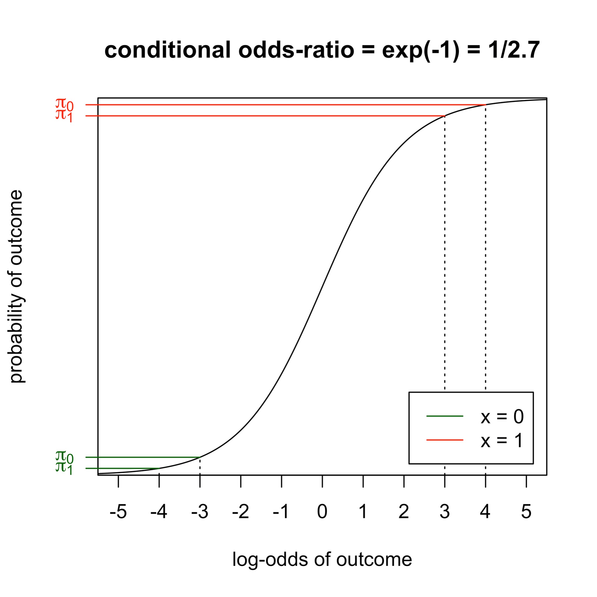
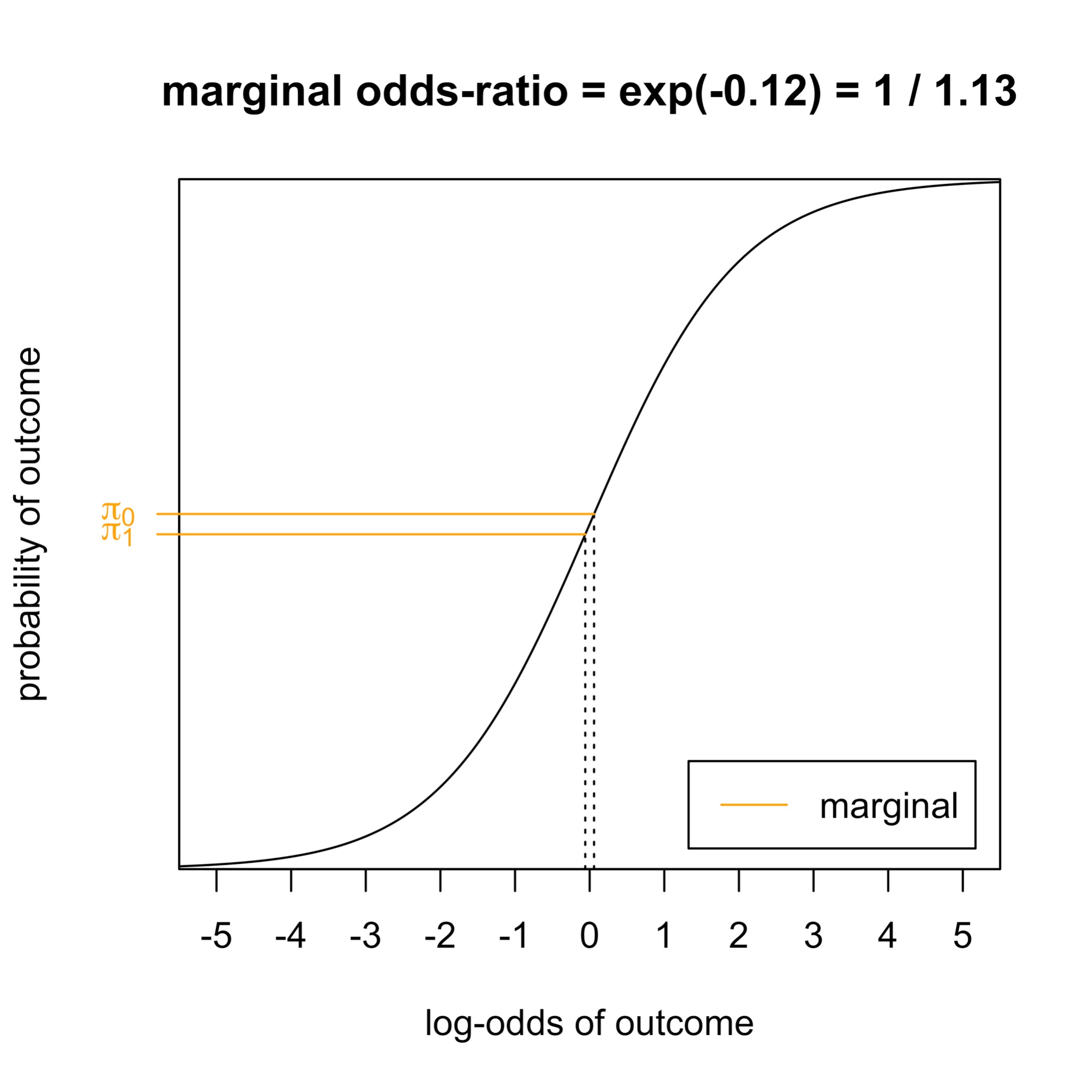
Non-collapsibility creates a mismatch
- The odds ratio for treatment depends on whether we condition on \(X\).
- This comes from the non-linearity of logistic regression.
- It also applies to hazard ratios.
- It gets stronger when \(X\) is a stronger outcome predictor.
Conundrum:
RCTs usually provide a marginal (log) odds ratio: \(\log \gamma = \log \frac{\text{odds}(E[Y_1])}{\text{odds}(E[Y_0])}\)
The offset model needs a conditional odds ratio.
The mismatch grows exactly when CATE variation becomes more useful.
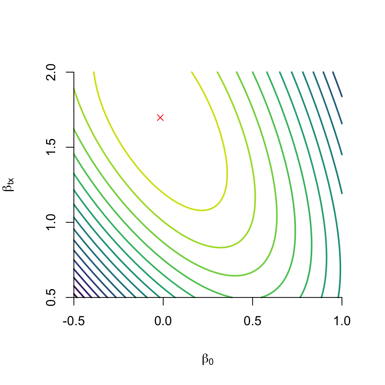
Fix: constrain the marginal odds ratio
Estimate all model parameters, including \(\beta_t\), but force the fitted model to reproduce the randomized marginal treatment effect in the target population.
- From trial: \(\gamma^* = \text{logit}(E[Y_1]) - \text{logit}(E[Y_0])\)
- For candidate model with parameters \(\theta\), compute:
\[ \begin{aligned} M_n(\theta) &=\mathrm{logit}\left\{\frac{1}{n}\sum_{i=1}^{n} P_\theta(Y=1\mid X=x_i,T=1)\right\} \\ &\quad-\mathrm{logit}\left\{\frac{1}{n}\sum_{i=1}^{n} P_\theta(Y=1\mid X=x_i,T=0)\right\}. \end{aligned} \]
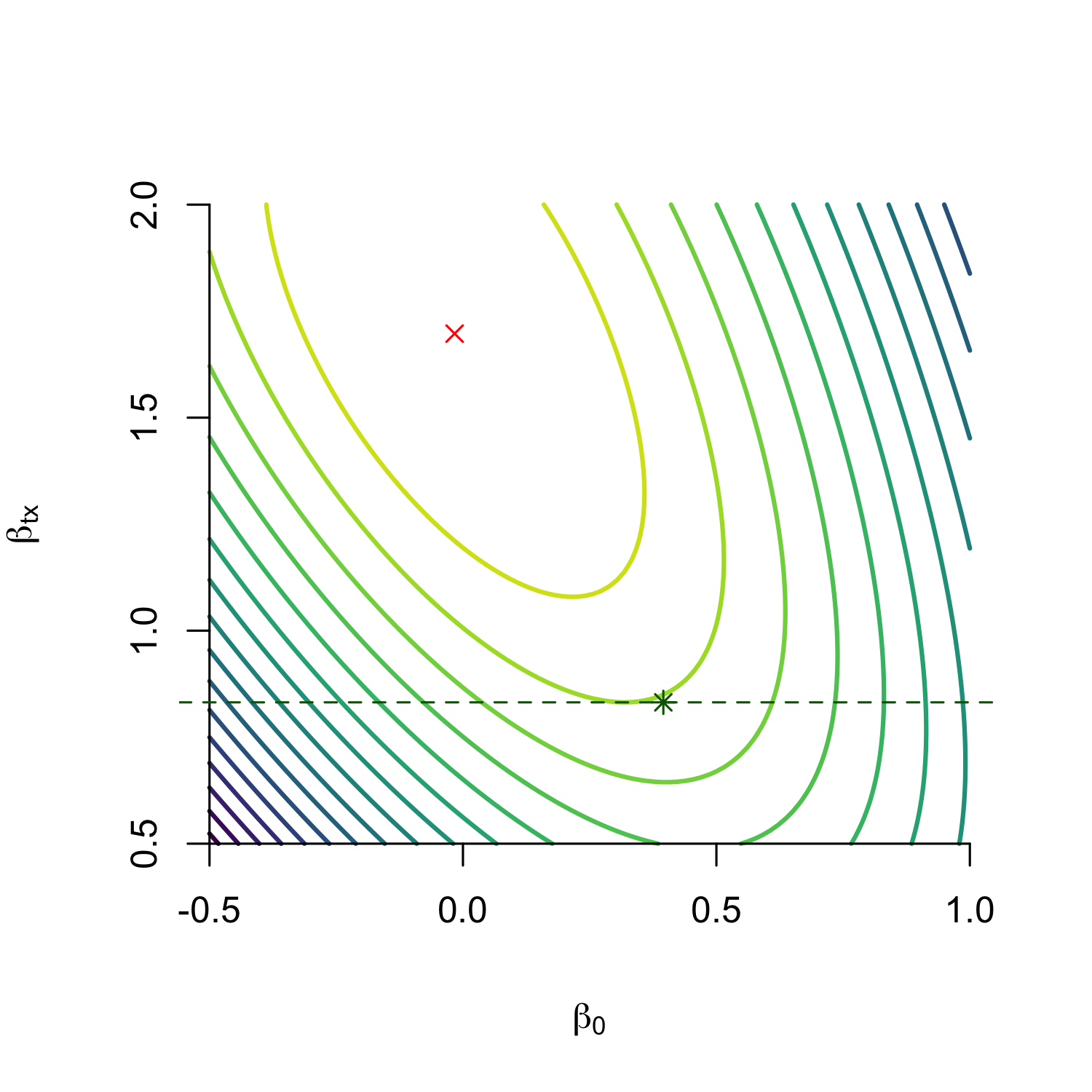
Marginally constrained objective
Fit the observational outcome model subject to:
\[ M_n(\theta) = \hat\gamma_{RCT}, \]
where \(\hat\gamma_{RCT}\) is the marginal log odds ratio reported by the trial.
Equivalently:
\[ \max_{\theta} \; \ell_{obs}(\theta) \quad \text{subject to} \quad M_n(\theta)-\hat\gamma_{RCT}=0. \]
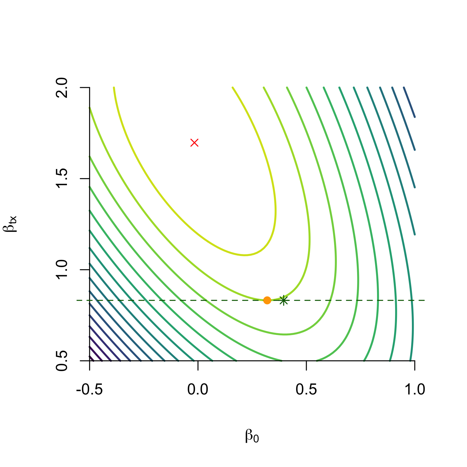
- We call such models marginally constrained models (MCM)
- When the model family assumes a constant relative treatment effect (here: \(\text{logit}^{-1}(P(Y=1|T,X)) = \beta_0 + \beta_x + \beta_t t\)), constant relative MCM (CR-MCM)
Intuition
The model can learn the conditional treatment coefficient that best explains the observational outcomes.
But it is only allowed to do so if the implied randomized experiment in the current population agrees with the trial evidence.
Why constrain the odds-ratio? Need a measure that is likely to be transportable between settings
Results
\[ \max_{\theta} \; \ell_{obs}(\theta) \quad \text{subject to} \quad M_n(\theta)-\hat\gamma_{RCT}=0. \]
- Theorem 1 (informal) under consistency, positivity and unconfoundedness and correct model specification, this is a consistent estimator of \(P(Y_t=1|X)\) and thus \(\tau(x)\)
- Efficiency: when compared to MCM, its unconstrained counterpart requires \(\approx\) 70-100% more observations to reach same width of confidence interval
How the constraint was implemented in the paper
The paper used an increasingly strong quadratic penalty:
\[ \ell_{obs}(\theta) - \lambda\{M_n(\theta)-\hat\gamma_{RCT}\}^2. \]
Algorithm:
- start with a small \(\lambda = 0.01\);
- optimize the unconstrained penalized objective with L-BFGS;
- check whether the constraint error is below \(10^{-4}\);
- multiply \(\lambda\) by 10 and repeat until satisfied.
This treats the trial estimate as effectively exact once the penalty becomes strong.
How much would all this matter in practice?
- aim was to estimate \(\tau(x)\)
- metric is mean squared error of \(\tau(x)\) (precision of estimated heterogeneous treatment effect):
\[\text{PEHE}(\hat{\tau}) = E_x [(\tau(x) - \hat{\tau(x)})^2]\]
- Remember we started with saying \(\text{ATE} = E[\tau(x)]\) can be a bad estimator of CATE.
- Easy to see that:
\[\text{PEHE}(\text{ATE}) = \text{Var}(\text{CATE})\]
- If no variance in CATE, ATE is the optimal estimator
- Mabye offset models are not ‘correct’, are they better than ATE?
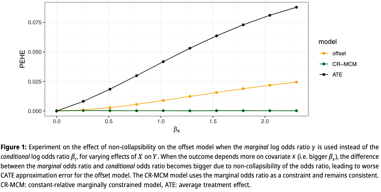
Result: PEHE under increasing non-collapsibility?
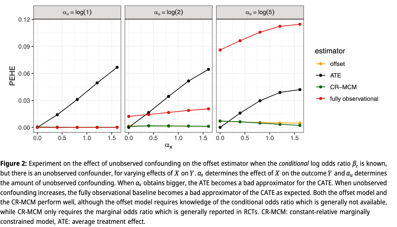
Result: when correct \(\beta_t\) is known but unobserved confounding
Bigger experiment
- \(X,T,U,Y\) binary
- \(T \sim p(T|U)\)
- \(Y \sim p(Y|T,X,U) = \text{logit}^{-1}(\alpha_0 + \alpha_x x + \alpha_t t + \alpha_u u)\)
- 12 dimensions, \(\geq 16*10^6\) experiments
- compare offset, MCM, CR-MCM
What’s the baseline?
- when \(\text{Var}(\text{CATE}) = 0, \text{PEHE}(\text{ATE}) = 0\)
- Consider as measure of how much PEHE can be gained:
\[\delta := | \text{CATE}(X=1) - \text{CATE}(X=0) | \]
- then when \(P(X=1) = 0.5\):
\[\text{Var}(\text{CATE}) = 0.25 \delta^2\]
Table 1: number of times method improves upon ATE in terms of PEHE
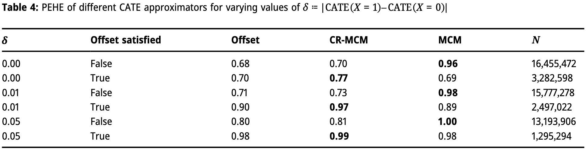
- when more variance in CATE, all methods perform better
- MCM performs best
- when offest (constant-relative) assumption holds, those methods work better
- standard offset often better under non-zero variance in CATE
Caveats
- compare on single metric across huge range of settings
- average performance, no gaurantee on single setting
Limitations and future work
- assumed direct transportability of marginal odds ratio
- in calculation of implied marginal odds-ratio, used unweighted sample average, could replace with importance weights based on \(X\) if known between trial and observational data if they have different covariate distributions
- we (silently) assumed knowing the marginal odds-ratio with infinete precision and no bias
- unpublished experiments show MCM rapidly worse than ‘fully observational’ when variance of RCT estimate (wrong constraint)
- better would be to consider uncertainty, e.g. as ‘Bayesian prior’:
\[ \ell_{obs}(\theta) - \frac{1}{2} \left( \frac{M_n(\theta)-\hat\gamma_{RCT}} {\mathrm{SE}(\hat\gamma_{RCT})} \right)^2. \]
Extensions
- are there better measures of effect to assume are constant? (e.g. risk ratio or survival ratio (Colnet et al. 2023))
- extend to Hazard Ratios (calculating constraint requires an optimization)
- what happens with higher dimensional \(X\)?
- investigate MCMs in applications
Take-home
- Offset models ask a reasonable clinical question: can trial relative effects turn prediction models into CATE models?
- The naive offset has two problems: confounding and marginal-versus-conditional effect mismatch.
- MCM uses the trial result as a marginal constraint, which is the scale on which trials often report evidence.
- The next estimator should treat the trial estimate as uncertain evidence, not an exact equality.
References
©Wouter van Amsterdam — WvanAmsterdam — wvanamsterdam.com/talks