PROTECT update

Manchester / Rajesh

Wouter van Amsterdam, MD, PhD

Department of Data Science Methods, Julius Center, University Medical Center Utrecht

2025-07-13

Updates in PROTECT methods

1. swap conditional hazard ratio with marginal hazard ratio

2. calculations for model checks

   1. correct marginalization incorporating prior likelihood of latent factor
   2. compare against cross-validated baseline likelihoods (not full-batch)

Conditional vs marginal hazard ratio

• realization: PROTECT models a conditional hazard ratio for treatment (conditional on latent factor, … some other variables)
• trials calculate a marginal hazard ratio
• these are incommensurable
• can calculate a marginal hazard ratio by simulating survival times from hypothetical trials using inferred parameters and patient data by setting treatment to 0 and 1 for every patient

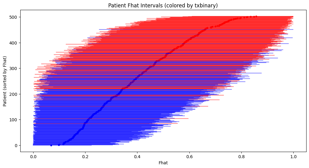
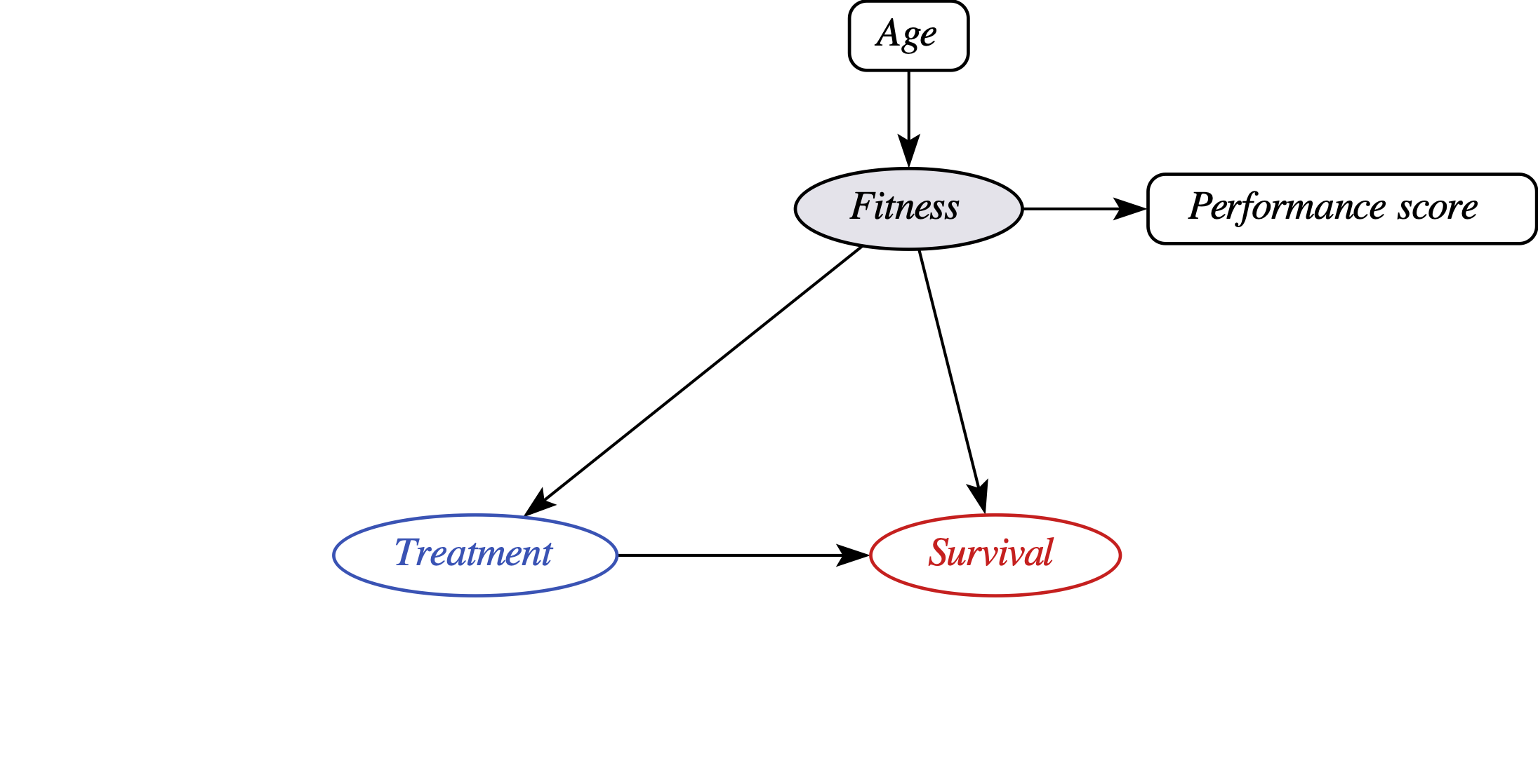
PROTECT uses a latent factor model for the unobserved confounder

• PROTECT models the joint likelihood of ‘observables’:
  • treatment \(T\), survival \(Y\) and proxies \(W\) of fitness (performance score, fraily)
  • … conditional on ‘controls’ \(X\) (age, stage, histology)
• in addition to ‘global parameters’ \(\theta\) that any regression model has (e.g. treatment to outcome regression coefficient), PROTECT has ‘local parameters’ (local to every patient \(i=1, ... N\)): \(F_i\)

PROTECT inference

• by running MCMC on the ‘training data’, we get samples from the posterior distribution over PROTECT’s parameters:

\[\begin{align*} p(\theta,F|T,Y,W,X) &\propto p(Y,T,W|X,\theta,F) p(F|X, \theta) p(\theta) \end{align*}\]

• in PROTECT, the joint likelihood is formulated as the product of the observation sites following the causal factorization:

\[\begin{align*} p(Y,T,W|X,\theta,F) = p(Y|T,X,\theta,F) p(T|X,\theta,F) p(W|X,\theta,F) \end{align*}\]

• during inference, the posterior for latent factor \(F_i\) of patient \(i\) is informed by their full observed data: \(X_i, W_i, T_i, Y_i\)

PROTECT model checks

• multiple models may be considered compatible with prior knowledge (in practice: different sets of priors)
• in Utrecht, we found for some priors PROTECT copied the treatment into the latent factor, leading to a violation of (a form of) positivity, and unidentifiedness of the treatment effect
• PROTECT has data-driven model checks to assess whether the latent factor ‘effectively communicates’ information between all its dependents (W, T, Y)
• for this, we need distributions over \(F\) using partial information (i.e. different ‘posterior predictive modes’), e.g. ‘no-\(Y\)’:

\[P(F_i|W_i,T_i,X_i,\theta = \theta_s)\]

• note that for every sample \(\theta_s\) of the posterior distribution of global parameters, this distirbution is different

Nested integratoin

\[P(F_i|W_i,T_i,X_i,\theta = \theta_s)\]

• to calculate predictive likelihoods, for example for \(Y\) given \(X,W,T\), we need to do nested integration:

\[\begin{align*} l(Y_i|X_i,W_i,T_i,\{\theta_s\}) &= \sum_s l(Y_i|X_i,W_i,T_i,\theta_s) \\ &= \sum_s \int_{-\infty}^{\infty}l(Y_i|X_i,W_i,T_i,f,\theta_s)p(f|T_i,W_i,X_i,\theta_s)df \end{align*}\]

Nested integration done right

• we need to numerically approximate the integrals
• this approximation should be unbiased and good enough to not be sensitive to e.g. the random seed for MCMC
• we can approximate by running separate MCMC for every sample \(\theta_s\), or a subset
• because this is effectively a large set of 1D integrals, can use faster approximation

approximation in original PROTECT

• take a grid of values for \(f\), for each value (and a given \(\theta_s\)), calculate the joint likelihood of the observables for that posterior predictive mode (e.g. \(W_i,T_i\))
• calculate the weighted sum of the log-likelihood of observed \(Y_i\), weighted by the joint likelihood of the \(F-\)conditioning observables
• omission: calculation did not weigh in the prior probability of \(f\), so the predictive likelihoods do not correspond to the actual PROTECT model

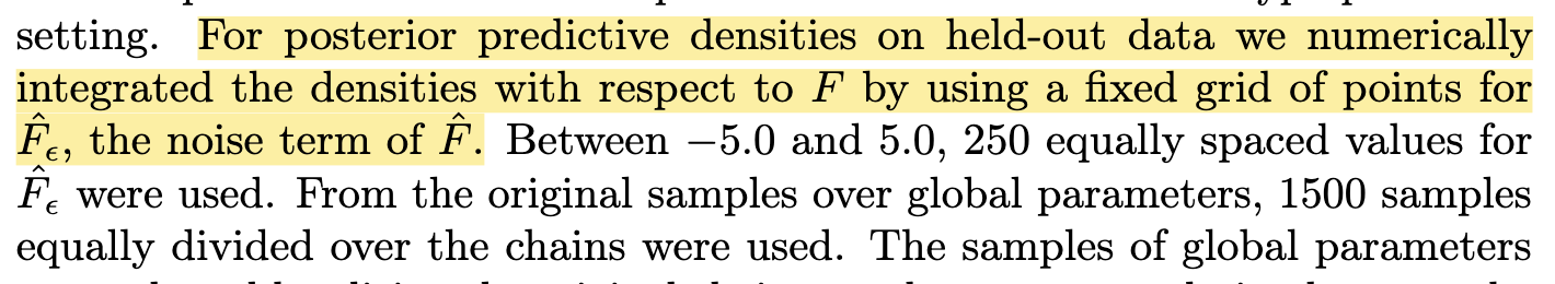
‘new’ solution: use Gauss-Hermite Quadrature

• to integrate over a gaussian distribution, pick \(K\) carefully chosen points \(X_k\) with corresponding weights \(W_k\)
• implemented in PROTECT library, consequences:
  • with much fewer points (\(K=32\)),
  • much better approximation,
  • incorporates prior over \(f\)
• the new approach is tested in cases with analytically knwon likelihoods (gaussian outcome and proxies)

By Qwfp - Own work, CC BY-SA 3.0, https://commons.wikimedia.org/w/index.php?curid=10803823

New Utrecht results

• rct: log(HR) -0.17
• before:
  • selected hyperparameters: s_bftx: 2.5, s_bfy: {0.1, 1.0, 2.5}
  • b_txbinary_y_marginal 0.010 (sd: 0.223, 95 hdi: -0.409 - 0.450)
• now:
  • selected hyperparameters:
    • sbftxs = np.array([0.1, 2.5, 10.0, 10.0, 100.0, 100.0])
    • sbfys = np.array([1.0, 1.0, 1.0, 2.5, 1.0, 2.5])
  • b_tx_y_marginal: 0.067 (sd: 0.229, 95 hdi: -0.356 - 0.525)
  • marginalized HR: 0.033 (sd: 0.20)

Utrecht overlap?