Causal perspectives on prediction modeling
2024-08-08
Recap: causal questions
- questions of association are of the kind:
- what is the probability of \(Y\) (potentially: after observing \(X\))?, for example:
- what is the chance of rain tomorrow given that is was dry today?
- what is the chance a patient with lung cancer lives more than 10% after diagnosis?
- these hands behind your back and passively observe the world-questions
- what is the probability of \(Y\) (potentially: after observing \(X\))?, for example:
- causal questions are of the kind:
- how would \(Y\) change when we intervene on \(T\)?, e.g.:
- if we would send all pregant women to the hospital for delivery, what would happen with neonatal outcomes?
- if we start a marketing campain, by how much would our revenue increase?
- these tell us what would happen if we changed something
- how would \(Y\) change when we intervene on \(T\)?, e.g.:
What is prediction? How does it compare to causal inference?
Examples of prediction tasks
observe an \(X\), want to know what to expect for \(Y\)
1. X = patient coughs, Y = patient has lung cancer
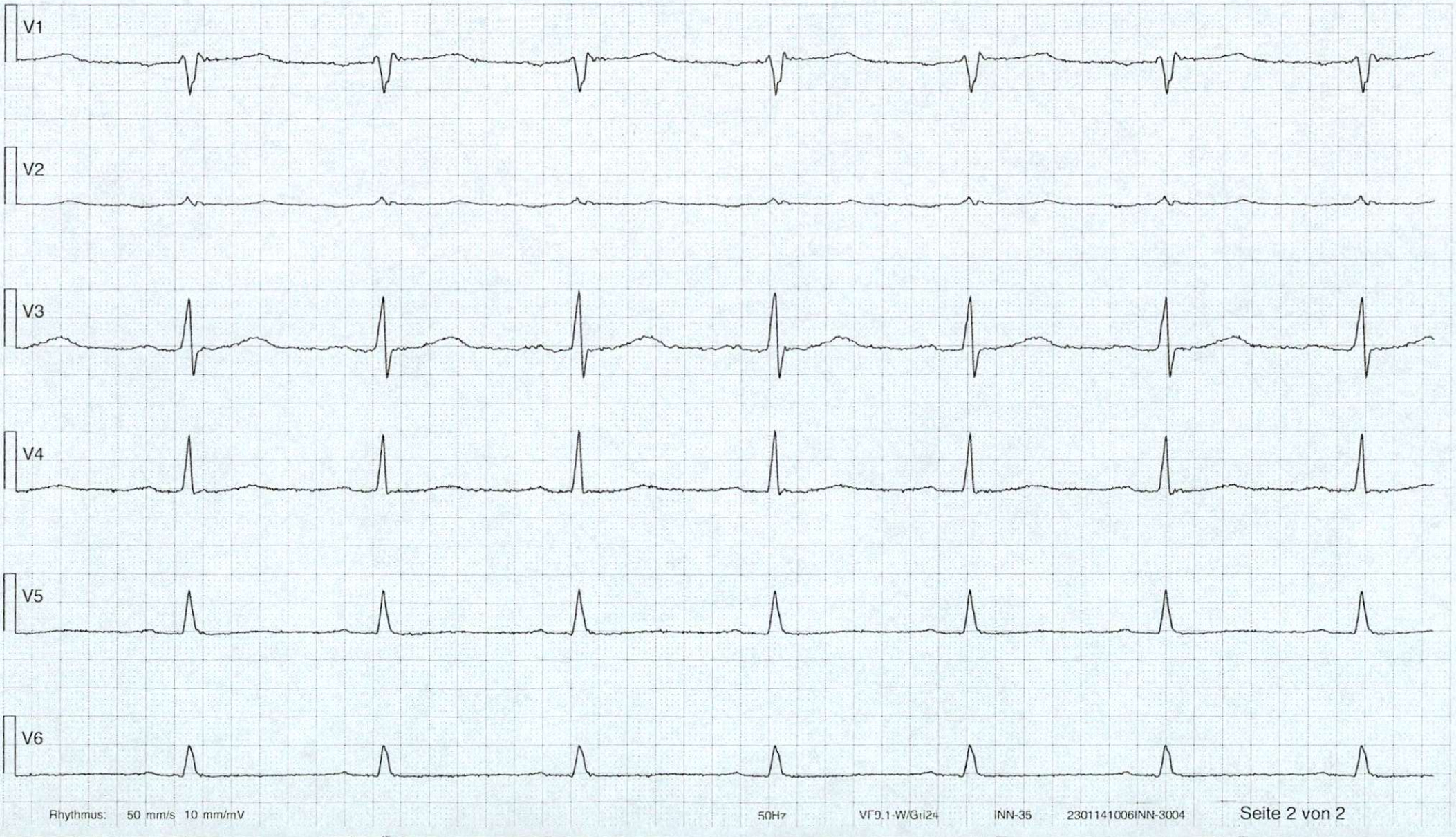
2. X = ECG, Y = patient has heart attack
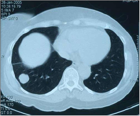
3. X = CT-scan, Y = patient dies within 2 years
Prediction: typical approach
- define population, find a cohort
- measure \(X\) at prediction baseline
- measure \(Y\)
- cross-sectional (e.g. diagnosis)
- longitudinal follow-up (e.g. survival)
- use a statistical learning technique (e.g. regression, machine learning)
- fit model \(f\) to observed \(\{x_i,y_i\}\) with a criterion / loss function
- evaluate prediction performance with e.g. discrimination, calibration, \(R^2\)
Prediction: typical estimand
Let \(f\) depend on parameter \(\theta\), prediction typically aims for:
\[f_{\theta}(x) \to E[Y|X=x]\]
- when \(Y\) is binary:
- probability of a heart attack in 10 years, given age and cholesterol
- probability of lung cancer, given symptoms and CT-scan
- typical evaluation metrics:
- discrimination: sensitivity, specificity, AUC
- calibration
Causal inference: typical approach
- define target population and targeted treatment comparison
- run randomized controlled trial, randomizing treatment allocation (when possible)
- measure patient outcomes
- estimate parameter that summarizes average treatment effect (ATE)
typical estimand:
\[E[Y|\text{do}(T=1)] - E[Y|\text{do}(T=0)]\]
Causal inference versus prediction
prediction
- typical estimand \(E[Y|X]\)
- typical study: longitudinal cohort
- typical interpretation: \(X\) predicts \(Y\)
- primary use: know what \(Y\) to expect when observing a new \(X\) assuming no change in joint distribution
causal inference
- typical estimand \(E[Y|\text{do}(T=1)] - E[Y|\text{do}(T=0)]\)
- typical study: RCT (or observational causal inference study)
- typical interpretation: causal effect of \(T\) on \(Y\)
- primary use: know what change in \(Y\) to expect when setting the treatment policy
Where can prediction and causality meet?
- prediction has a causal interpretation
- prediction may or may not have a causal interpretation:
- but is used for a causal task (e.g. treatment decision making)
- but predictions can be improved with causal thinking in terms of e.g.:
- interpretability, robustness, ‘spurious correlations’, generalization, fairness, selection bias
1. Prediction has a causal interpretation
What can we mean with predictions having a causal interpretation?
Let \(f: \mathbb{X} \to \mathbb{Y}\) be a prediction model for outcome \(Y\) using features \(X\)
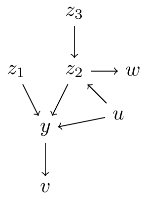
- \(X\) is an ancestor of \(Y\) (\(X=\{z_1,z_2,z_3\}\))
- \(X\) is a direct cause of \(Y\) (\(X=\{z_1,z_2\}\))
- \(f: \mathbb{X} \to \mathbb{Y}\) describes the causal effect of \(X\) on \(Y\) (\(X=\{z_1\}\)), i.e.:
\[f(x) = E[Y|\text{do}(X=x)]\]
- \(f: \mathbb{T} \times \mathbb{X} \to \mathbb{Y}\) describes the causal effect of \(T\) on \(Y\) conditional on \(X\) (\(T=\{z_1\},X=\{z_2,z_3,w\}\)):
\[f(t,x) = E[Y|\text{do}(T=t),X=x]\]
interpretation 3. all covariates are causal
Let \(f: \mathbb{X} \to \mathbb{Y}\) be a prediction model for outcome \(Y\) using features \(X\)
\[f(x) = E[Y|\text{do}(X=x)]\]
- the requirements for this interpretation are very hard to satisfy (i.e. back-door rule holds for all variables)
- too often this is assumed / interpreted this way (table 2 fallacy in health care literature)
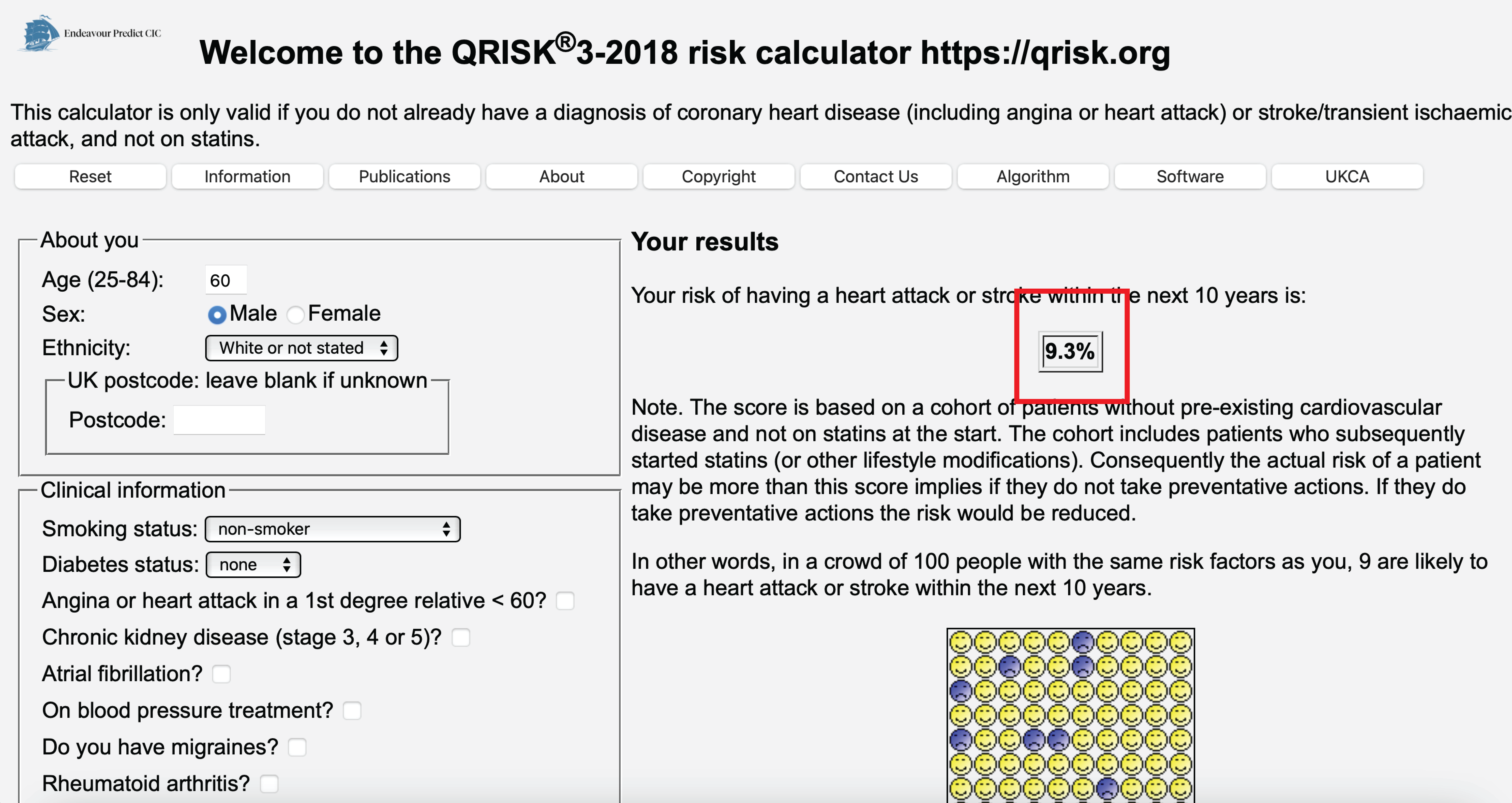
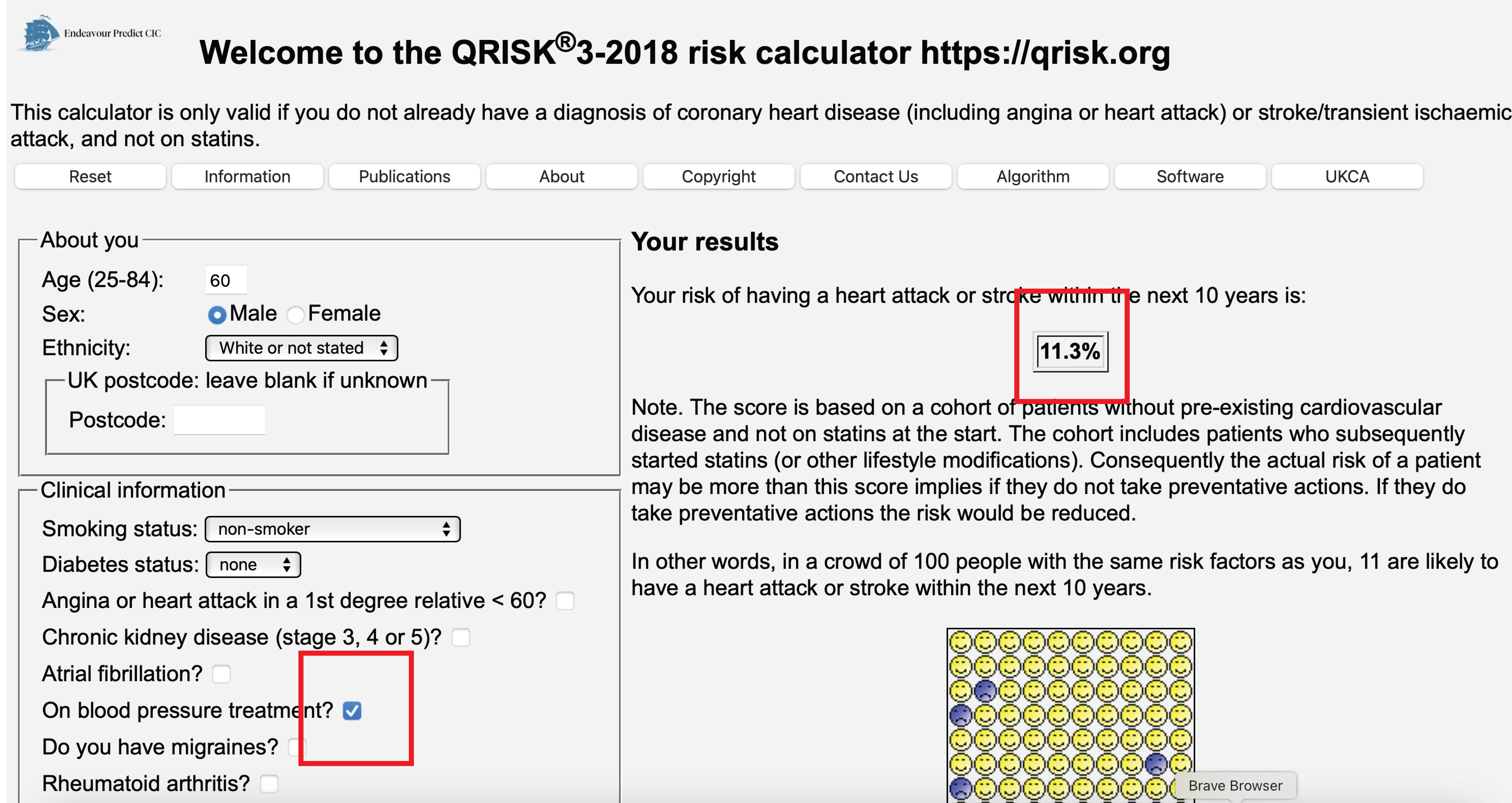
Example of table 2 fallacy when mis-using Qrisk
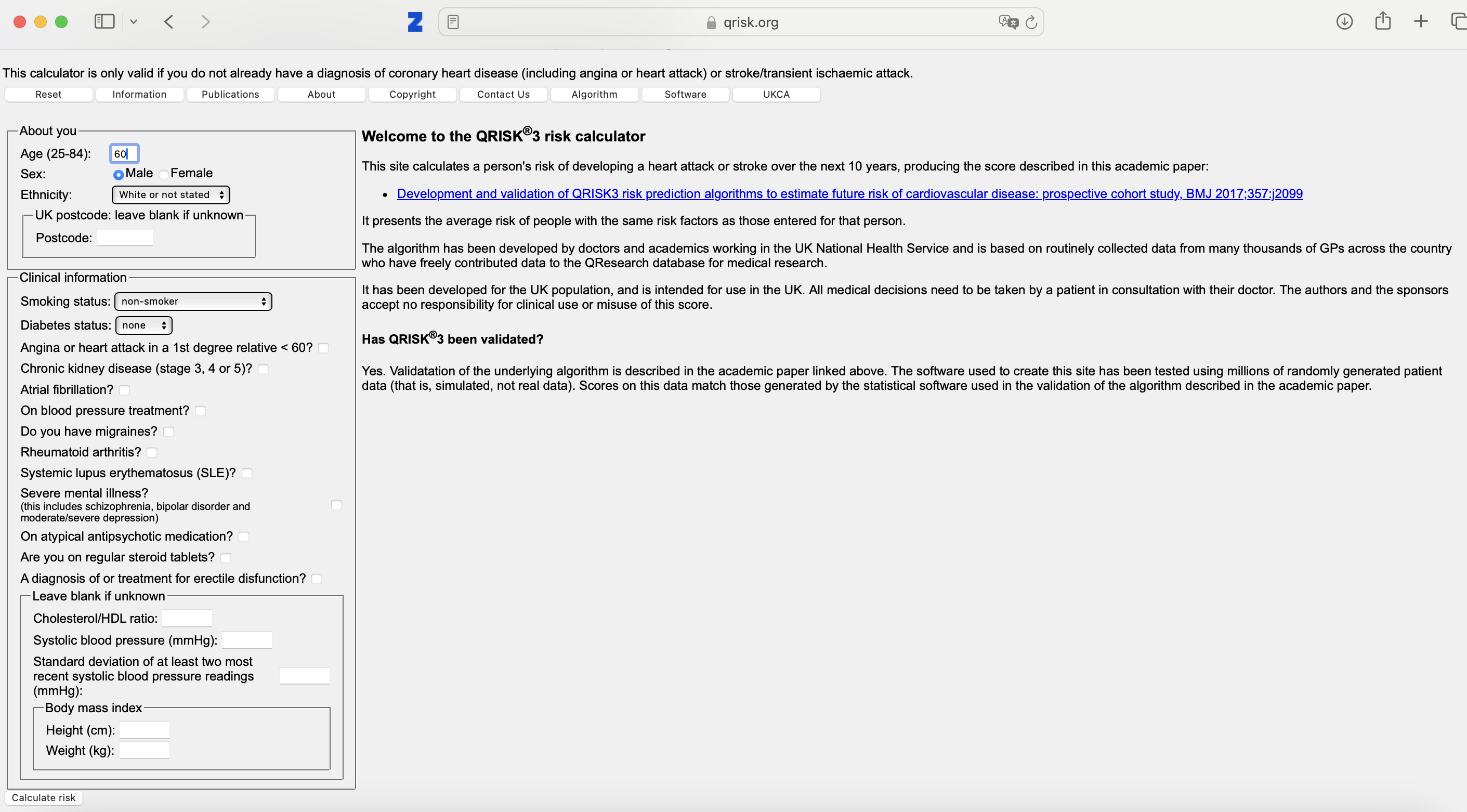
Qrisk3: a risk prediction model for cardiovascular events in the coming 10-years. Widely used in the United Kingdom for deciding which patients should get statins
Qrisk3 - risks:
can go wrong when:
- e.g. fill in current length and weight
- reduce weight by 5 kgs
- interpret difference as ‘effect of weight loss’
- check or un-check blood pressure medication
- observe that with blood pressure medication, risk is higher
interpretation 4. some covariates are causal
or: prediction-under-intervention
\[f(t,x) = E[Y|\text{do}(T=t),X=x]\]
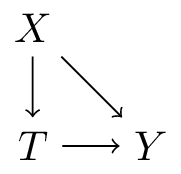
- interpretation: what is the expected value of \(Y\) if we were to assign treatment \(t\) by intervention, given that we know \(X=x\) in this patient
Estimand for prediction-under-intervention models
What is the estimand?
- prediction: \(E[Y|X]\)
- average treatment effect: \(E[Y|\text{do}(T=1)] - E[Y|\text{do}(T=0)]\)
- conditional average treatment effect: \(E[Y|\text{do}(T=1),X] - E[Y|\text{do}(T=0),X]\)
- prediction-under-intervention: \(E[Y|\text{do}(T=t),X]\)
note:
- from prediction-under-intervention models, the CATE can be derived
- in these models and the CATE: \(T\) has a causal interpretation, \(X\) does not!
- i.e. \(X\) does not cause the effect of treatment to be different
Developing prediction-under-intervention models
requires causal inference assumptions or RCTs
single RCTs often not big enough, or did not measure the right \(X\)s
when \(X\) is not a sufficient adjustment set, but \(X+L\) is, can adjust additionally for \(L\) using e.g. propensity score methods or standardization
assumption of no unobserved confounding often hard to justify in observational data
but there’s more between heaven (RCT) and earth (confounder adjustment)
- proxy-variable methods (e.g. Miao et al. 2018; van Amsterdam et al. 2022)
- constant relative treatment effect assumption (e.g. Alaa et al. 2021; van Amsterdam and Ranganath 2023; Candido dos Reis et al. 2017)
- diff-in-diff
- instrumental variable analysis (Wald 1940; Puli and Ranganath 2021; Hartford et al. 2017)
- front-door analysis
not covered now: formulating correct estimands (and getting the right data) becomes much more complicated when considering dynamic treatment decision processes (e.g. blood pressure control with multiple follow-up visits) (Luijken et al. 2024)
Evaluating predictive performance of prediction-under-intervention models
- Estimand for prediction-under-intervention: expected outcome under intervention, conditional on covariates \(X\)
- prediction accuracy can be tested in RCTs, this is the target distribution
- or in observational data with specialized methods accounting for confounding (e.g. (Boyer et al. 2025; Keogh and van Geloven 2024))
- remember from Day 2: observational causal inference is using data we have and assumptions to make inferences about a setting on which we do not have data
- in confounded observational data, typical metrics (e.g. AUC or calibration) are not sufficient as we want to predict well in data from other distribution than observed data (i.e. other treatment decisions)
- evaluation approaches based on confounder adjustment methods:
- IPW reweighting
- confounder adjustment / standardization
- doubly robust methods
2a. (Prediction) models used for a causal task (decision making)
Using prediction models for decision making is often thought of as a good idea
For example:
- give chemotherapy to cancer patients with high predicted risk of recurrence
- give statins to patients with a high risk of a heart attack
TRIPOD+AI on prediction models (Collins et al. 2024)
“Their primary use is to support clinical decision making, such as … initiate treatment or lifestyle changes.”
- in abstract terms: prediction model \(f\) induces a new treatment policy
What do we mean with treatment policy?
A treatment policy \(\pi\) is a procedure for determining the treatment
Assuming \(T\) is binary, \(\pi\) can be:
- \(\pi = 0.5\) (a 1/1 RCT)
- deterministic guideline, e.g. give blood pressure pill to patients with hypertension:
\[\pi(\text{blood pressure}) = \begin{cases} 1, &\text{blood pressure} > 140\text{mmHg}\\ 0, &\text{otherwise} \end{cases}\]
- dependent on prediction models: give statins to patients with more than 10% predicted risk of heart attack; take \(f(X)\) as a prediction model for the risk of heart attack:
\[\pi(X) = \begin{cases} 1, &f(X) > 0.1\\ 0, &\text{otherwise} \end{cases}\]
- the propensity score is an estimate of the current treatment policy, conditional on features \(X\):
\[\pi_0(X) = P(T=1|X)\]
Let’s think about old and new treatment policies
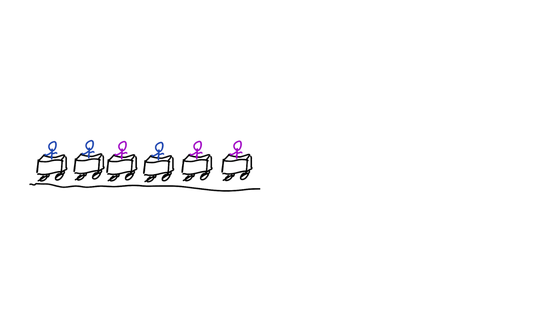
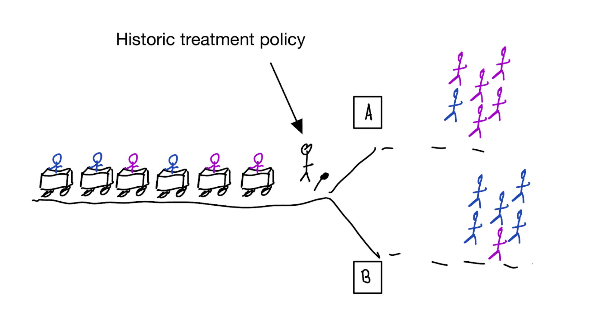
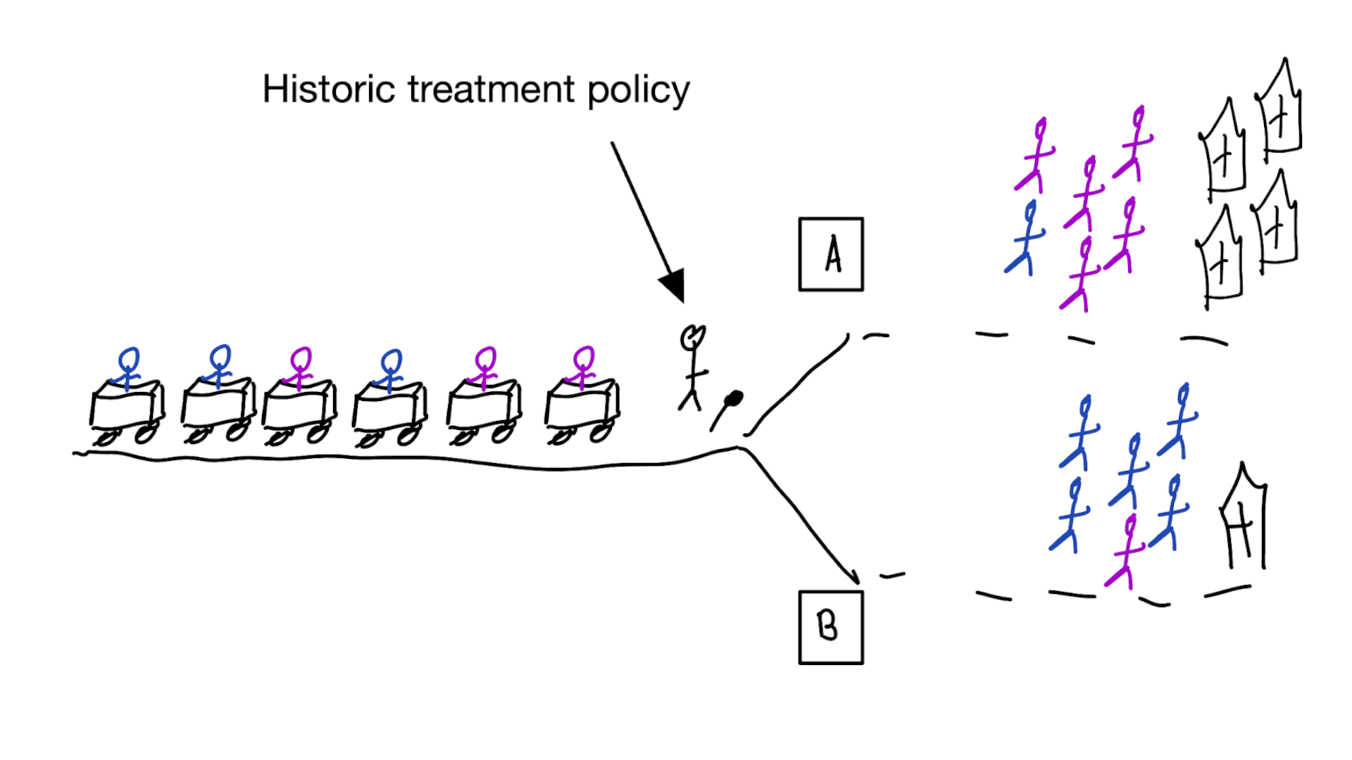
Model deployment is an intervention, changing treatments and outcomes
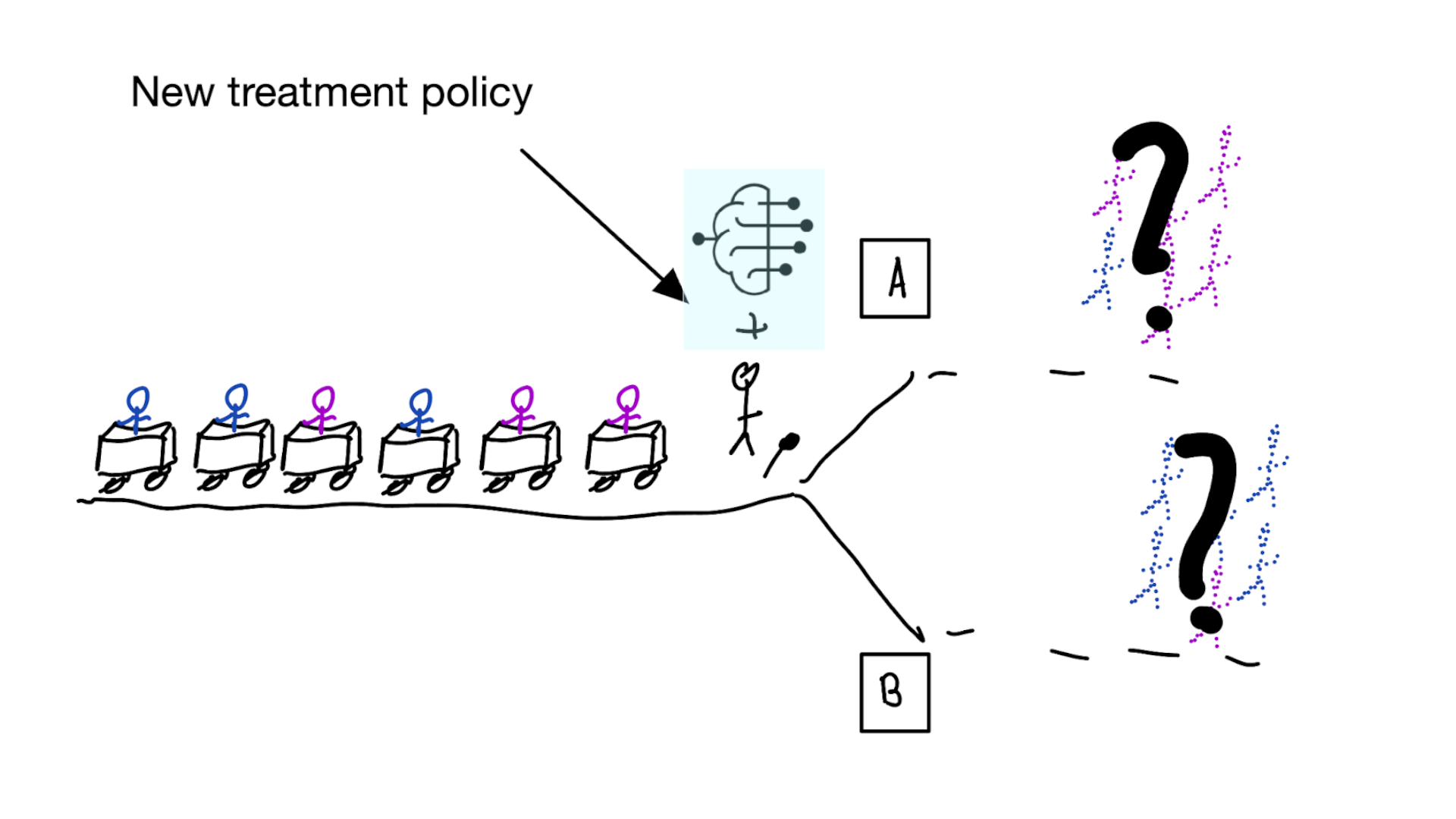
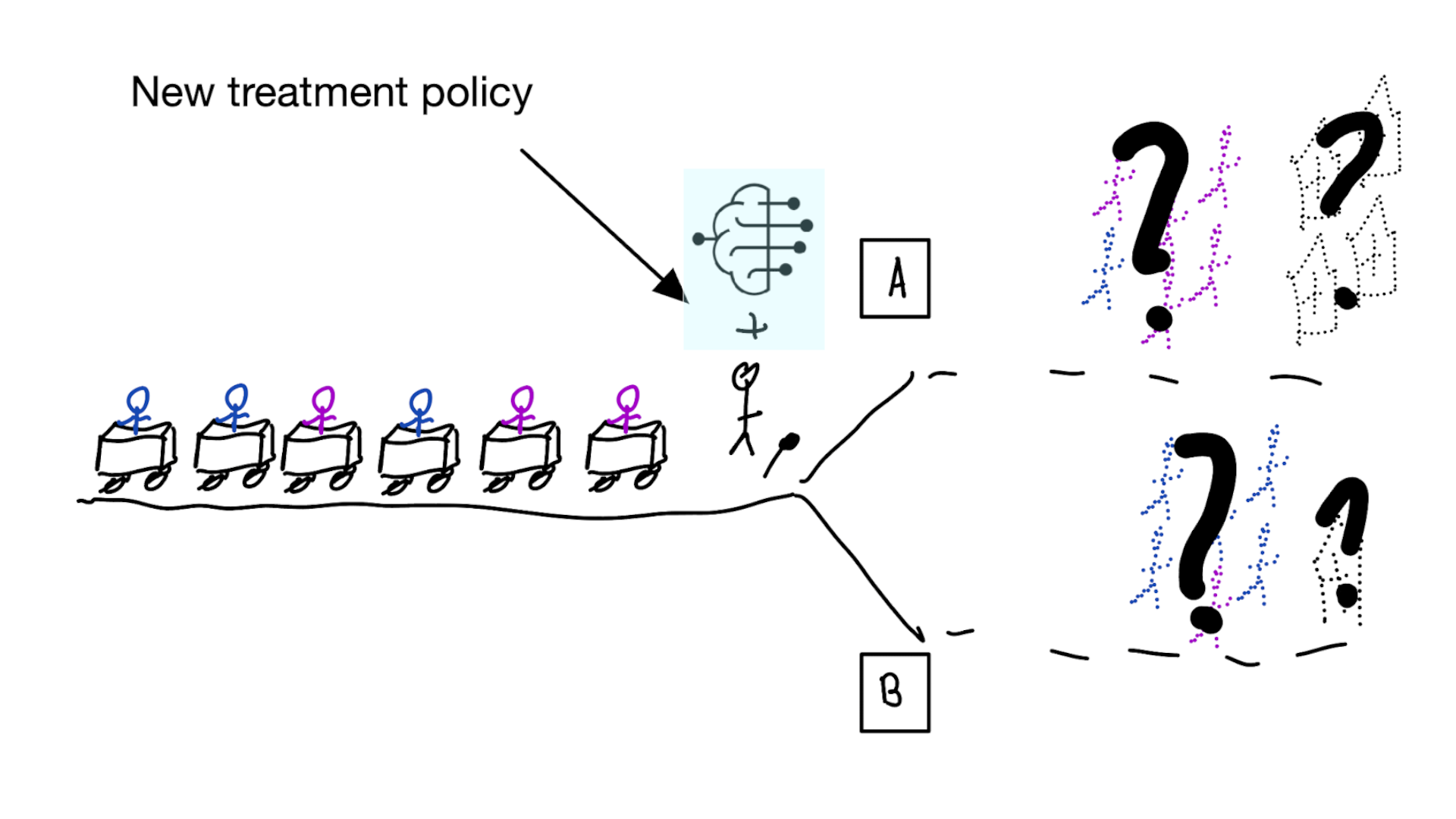
How do we learn about the effect of an intervention?
With causal inference!
- for using a decision support model, the unit of intervention is the decision maker, typically a healthcare provider
- randomly assign providers to have access to the model or not
- measure differences in treatment decisions and patient outcomes
- this called a cluster RCT: outcomes on patient level, who clustered within randomized units (e.g. healthcare providers, hospitals, schools, etc.)
- if using model improves outcomes, use that one
Using cluster RCTs to evaluated models for decision making is not a new idea (Cooper et al. 1997)
“As one possibility, suppose that a trial is performed in which clinicians are randomized either to have or not to have access to such a decision aid in making decisions about where to treat patients who present with pneumonia.”
What we don’t learn
was the model predicting anything sensible?
What if we cannot do this (cluster randomized) trial?
Off-policy evaluation
- What we want to know: what is expected value of \(Y\) under a new treatment policy \(\pi_1\)?
- have historic RCT data, want to evaluate new policy \(\pi_1\)
- when \(\pi_1(x)\) is deterministic (e.g. give the treatment when \(f(x) > 0.1\)), we get the following:
- when randomized treatment is concordant with \(\pi_1\), keep the patient, otherwise, remove from the data
- calculate average outcomes in the kept patients
- this way, multiple alternative policies may be evaluated
- when \(\pi_1(x)\) is deterministic (e.g. give the treatment when \(f(x) > 0.1\)), we get the following:
What if we cannot do this (cluster randomized) trial?
Off-policy evaluation in observational data
- have historic observational data, want to evaluate new policy \(\pi_1\):
- target distribution \(p(t|x)=\pi_1(x)\)
- observed distribution \(q(t|x) = \pi_0(x)\)
- we need to estimate \(q\) (i.e. the propensity score), this procedure relies on the standard causal inference assumptions (no confounding, positivity)
- every patient gets a weight \(w = \frac{\pi_1(x)}{\pi_0(x)}\) (i.e. the ratio of the target and observed treatment policy)
- calculate weighted average outcomes in the observed data
- (aka “importance sampling” in statistics / machine learning)
Off-policy evaluation limitations:
- typically requires a lot of data as:
- either many patients are concordant with the new policy, so small differences
- many discordant patients, so down-weighted and small effective sample size
What if we don’t know a threshold a-priori? Rank-based treatment allocation
RATE setup: evaluate a fixed prioritization rule
Take a model or rule \(f:\mathbb{X}\to\mathbb{R}\) as given.
- \(f\) could be a risk model, CATE model, clinical score, or hand-crafted rule
- larger \(f(x)\) means higher priority for treatment
- only the ranking matters; the numeric scale of \(f(x)\) does not
- evaluation asks whether treating higher-ranked patients first improves outcomes
- no requirement that \(f\) was trained to predict treatment effects
Turn ranks into treatment-allocation policies
For each treatment budget \(u\in[0,1]\), treat the top \(u\) fraction according to \(f\).
\[ \pi_{f,u}(x)=\mathbf{1}\{f(x)\ge q_{1-u}\} \]
where \(q_{1-u}\) is the \((1-u)\)-quantile of \(f(X)\).
- \(u=0\): treat nobody
- \(u=0.10\): treat the highest-ranked 10%
- \(u=1\): treat everybody
- sweeping \(u\) from 0 to 1 gives a sequence of rank-based policies
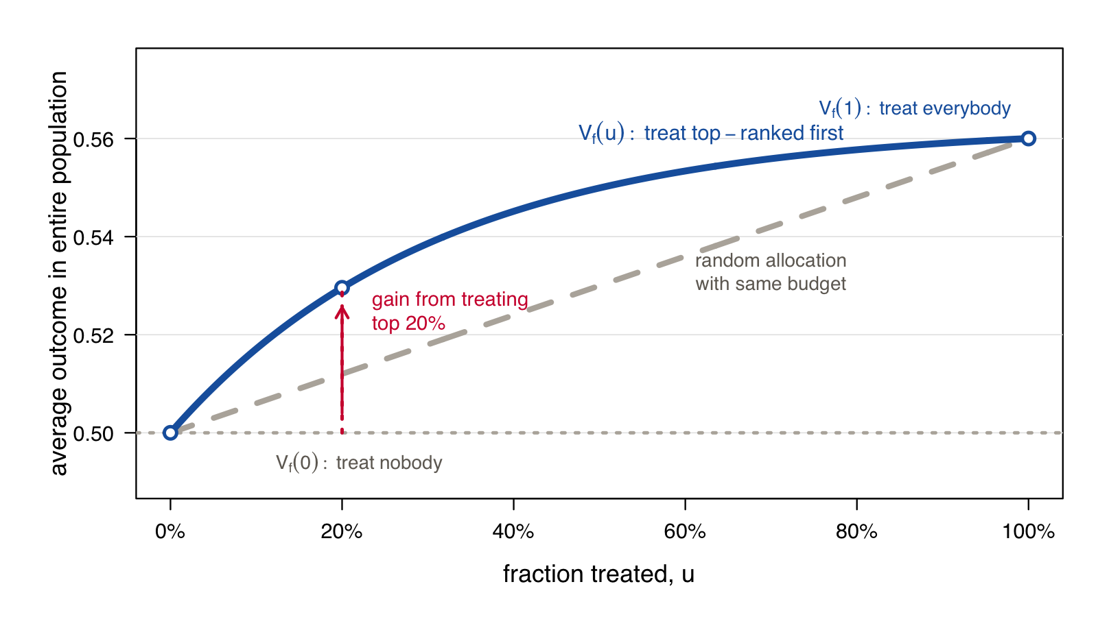
Start with the incremental policy-value curve
For this section, let larger \(Y\) mean better outcomes. Flip signs if \(Y\) is a harm.
\[ V_f(u)=E\left[\pi_{f,u}(X)Y(1)+\{1-\pi_{f,u}(X)\}Y(0)\right] \]
- x-axis: fraction of the population treated, \(u\)
- y-axis: average outcome in the entire population under policy \(\pi_{f,u}\)
- \(V_f(0)=E[Y(0)]\): nobody treated
- \(V_f(1)=E[Y(1)]\): everybody treated
- the curve answers: what average outcome would we get if treatment capacity were 5%, 10%, 20%, …
Visualizing the policy-value curve
Estimating the curve in evaluation data
In a randomized evaluation set with treatment probability \(e_i=P(T_i=1\mid X_i)\):
\[ \widehat{V}_f(u)=\frac{1}{n}\sum_{i=1}^n \left[ \frac{\pi_{f,u}(X_i)T_iY_i}{e_i} + \frac{\{1-\pi_{f,u}(X_i)\}(1-T_i)Y_i}{1-e_i} \right] \]
- score everyone with the fixed \(f\)
- sort from high to low priority
- for each \(u\), estimate the mean outcome if top-ranked patients were treated and the rest were not
- in observational data, this becomes causal evaluation: propensity weighting, standardization, or doubly robust estimators, plus the usual assumptions
- this is the same procedure as in off-policy evaluation, but now the policy is rank-based
Summarize the curve with RATE
RATE metrics are weighted areas under the TOC curve:
\[ \operatorname{RATE}_{\alpha}(f)=\int_0^1\alpha(u)\operatorname{TOC}_f(u)\,du \]
- AUTOC: \(\alpha(u)=1\)
- Qini coefficient: \(\alpha(u)=u\)
- choose \(\alpha\) based on which treatment budgets matter most
- RATE evaluates a ranking, not calibrated treatment-effect predictions
- use held-out or cross-fitted evaluation data; otherwise the curve can overstate value
c-for-benefit: concordance for predicted benefit
c-for-benefit is another rank-based evaluation summary, but for a fixed benefit score \(f\) (Hoogland et al. 2023).
- match treated and untreated patients into pairs that are similar in covariates or predicted benefit
- for pair with treated member and untreated member, pair is concordant if the member with better observed outcome also had larger predicted ‘benefit’
- compare all pairs, compute fraction of concordant pairs
Some warnings on bad evaluations
Prediction model types
- treatment-naive prediction models: \(E[Y|X]\)
- confounded (post-decision) prediction models: \(E[Y|X,T] \neq E[Y|X,\text{do}(T)]\)
- prediction-under-intervention models: \(E[Y|\text{do}(T),X]\)
Treatment-naive prediction models ignore the historic treatment policy
And can lead to bad situations like self-fulfilling prophecies (Van Amsterdam et al. 2025)
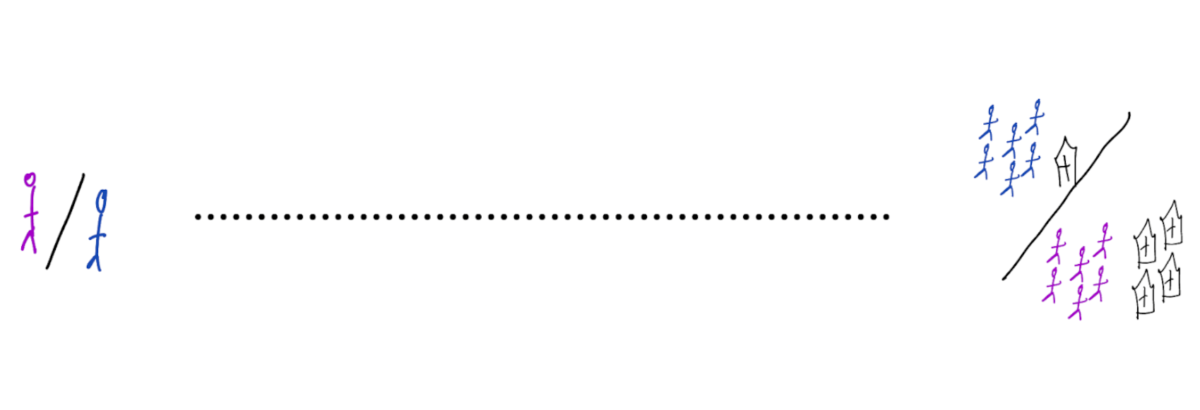
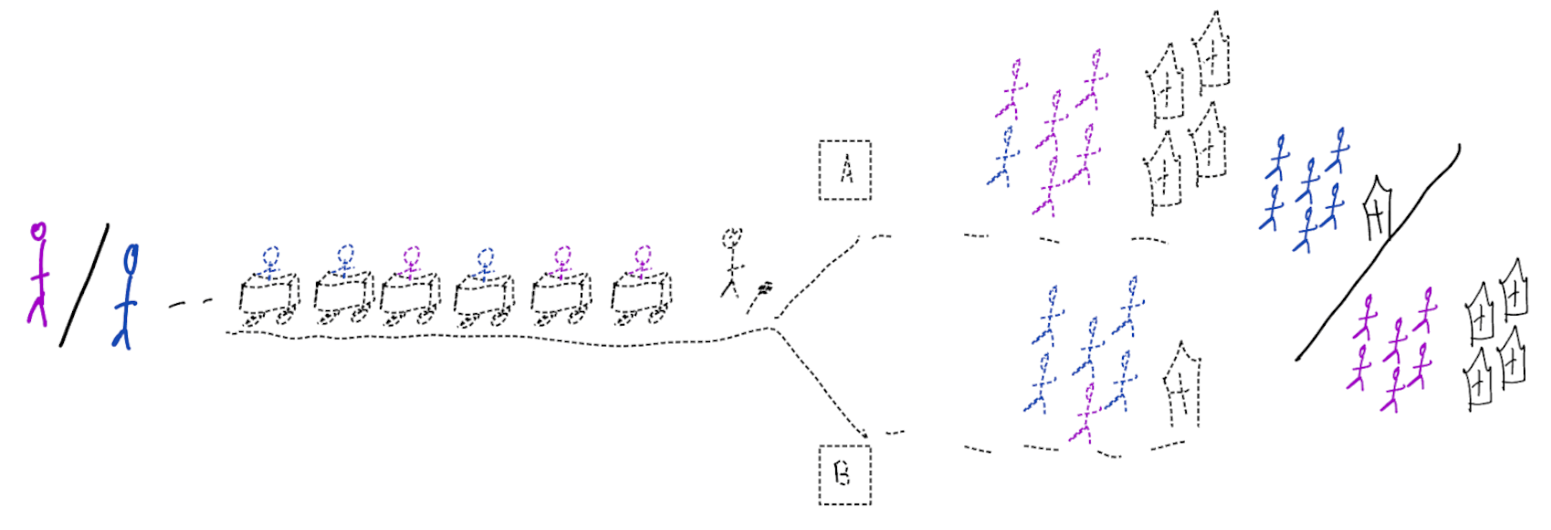
\[\begin{align} E[Y|X] \class{fragment}{= E[E_{t~\sim \pi_0(X)}[Y|X,t]]} \end{align}\]
Confounded prediction models do not account for confounding
Prediction under intervention models
- When correctly estimated, decision rule “give treatment with best predicted outcome” leads to foreseeable improvements.
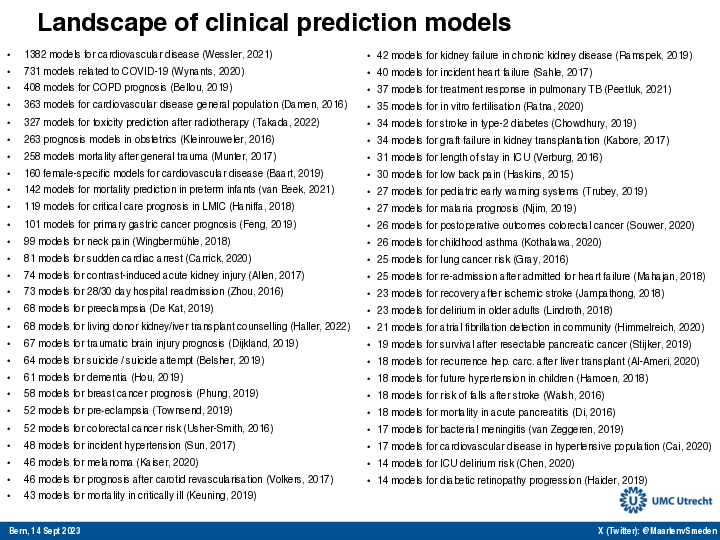
Prediction modeling is very popular in medical research
Recommended validation practices and reporting guidelines do not protect against harm
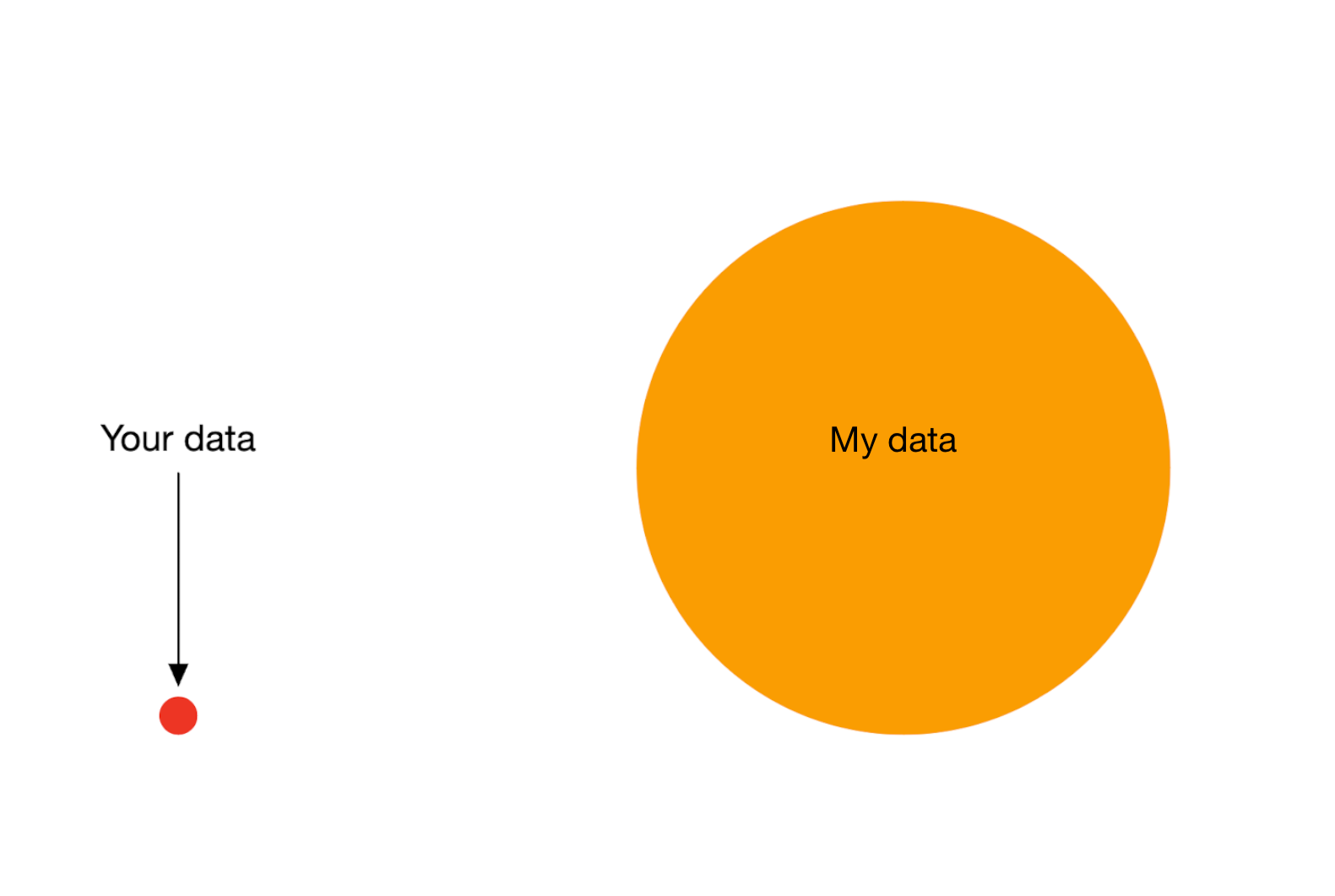
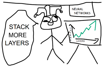
because they do not evaluate the policy change

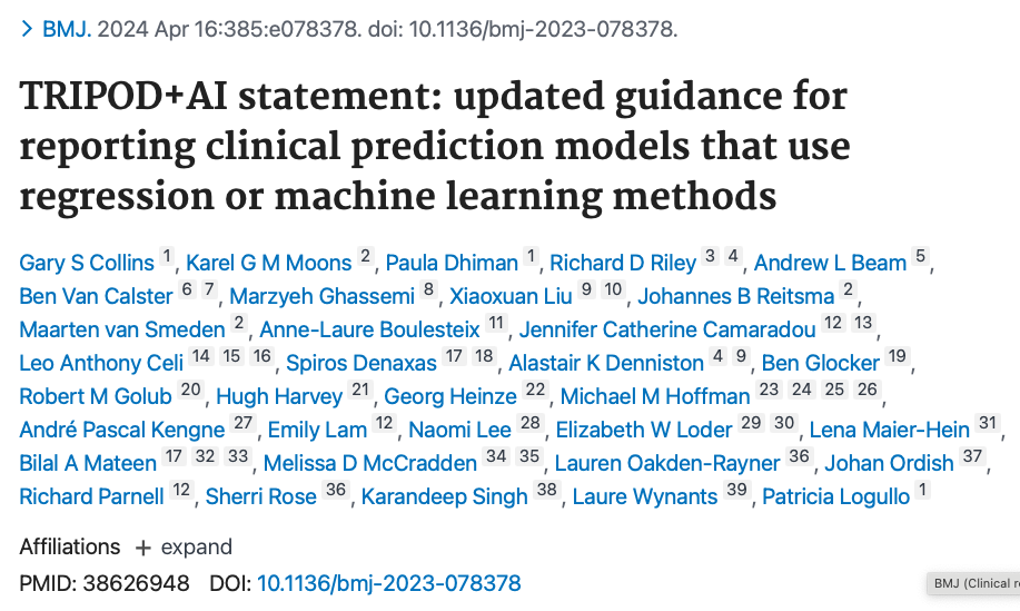
Bigger data does not protect against harmful prediction models
More flexible models do not protect against harmful prediction models
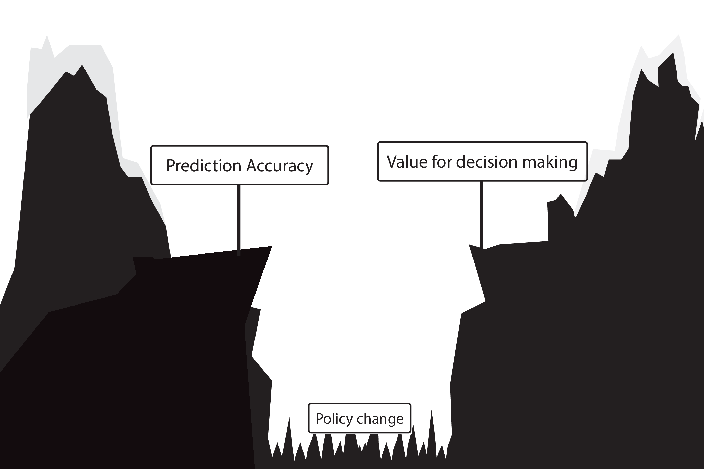
What to do?
What to do?
- Evaluate policy change (cluster randomized controlled trial)
- Build models that are likely to have value for decision making
2b. improving non-causal prediction models with causality
- interpretability
- robustness / ‘spurious correlations’ / generalization
- fairness
- selection bias
Interpretability
- end-users (e.g. doctors) often want to understand why a prediction model returns a certain prediction
- this has two possible interpretations:
- explain the model (i.e. the computations)
- explain the world (i.e. why is this patient at high risk of a certain outcome)
- often has a causal connotation, though achieving this is may be unfeasible as you need causal assumptions on all covariates (rember table 2 fallacy)
Robustness / spurious correlations / generalization
- prediction models are developed in some data, but are intended to be used elsewhere (in location, time, other)
- in causal language, shifts in distributions can be denoted as interventions on specific nodes
- prediction models that include (direct) causes may be more robust to changes as the chain between \(X\) and \(Y\) is shorter
- some machine learning algorithms like deep learning are very good at detecting ‘background’ signals, e.g.:
- cows typically stand on grass, so a model may use the grass to predict cows
- detect the scanner type from a CT-scanner
- if hospital A has scanner type 1 and hospital B has scanner type 2
- and the outcome rates differ between the hospitals, models may (mis)use the scanner type to predict the outcome
- what will the model predict in hospital C? or when A or B buy a scanner of different type?
- may be preventable with causality
Fairness
- in the historic distribution, outcomes may be affected by unequal treatment of certain demographic groups
- instead of perpetuating inequities, we may want to design models that diminish them
- this means intervening in the distribution (= a causal task)
- causality has a strong vocabulary for formalizing fairness
- actually achieving fairness is highly non-trivial, not in the least part due to unclear definitions
- chosing to not include sensitive attributes in a prediction model is often not gauranteed to improve fairness
Selection bias
- have samples from some selected subpopulation
- university hospital
- older men
- want to generalize to another subpopulation
- general practitioner
- younger women
- use DAGs to express the difference between source and target population
- calculate e.g. expected performance on target population with techniques like importance sampling
Wrap-up
- predictions can have causal interpretations
- prediction-under-intervention: causal with respect to treatment (not covariates)
- mis-use of non-causal models for causal tasks (e.g. prediction model for treatment decisions) is perilous
- always think about the policy change and its effect on outcomes
- evaluate policy changes with cluster RCTs, or historic RCTs and importance sampling
- causal thinking may improve other aspects of non-causal prediction models such as robustness, fairness, generalization
Proof of importance sampling unbiasedness
assuming \(x\) is discrete, otherwise replace sums with integrals for continuous \(x\)
want to compute the expected value of \(g(x)\) over distribution \(p\), but we have samples from another distribution \(x \sim q\)
\[E_{x \sim q} \left[ \frac{p(x)}{q(x)} g(x) \right] = \sum_x q(x) \left( \frac{p(x)}{q(x)} g(x) \right) = \sum_x p(x) g(x) = E_{x \sim p} \left[g(x) \right]\]
this assumes \(q(x)>0\) whenever \(p(x)>0\) for the ratio \(p/q\) to be defined
References